The color of noises

Foreword

For once, and as usual, I’d like to start by briefly telling you how I came to be interested in the subject of this article.
A day like any other. I’m about to go to bed when I hear a faint, high-pitched noise.
I spend a while looking for where this noise is coming from. Unable to find its source, I decide to put in earplugs before getting into bed.
What I wasn’t expecting is that instead of fading, the noise got louder. That’s when I realize something: the noise is inside my head.

For two years now, I’ve had what is called a persistent tinnitus.

Tinnitus

Although it isn’t the main topic of this article, let’s dwell on tinnitus for a moment.

Ameli definition (the French national health insurance): Tinnitus is the perception of noises (ringing, buzzing, hissing, etc.) heard in one ear (or both) or inside the head, without them having been emitted by any source in the outside world. These symptoms are often linked to acoustic trauma or to the aging of the ear.

Most people have already experienced it at least once. In the vast majority of cases, it’s temporary.
However, it can sometimes become permanent.
This is often the case after prolonged exposure to an excessively loud sound without protection, but it can also appear spontaneously overnight (as it did for me).

In 95% of cases, the sound of the tinnitus doesn’t come from an external source, it’s only perceived by the brain. This is called subjective tinnitus.
In the remaining 5%, it’s said to be objective: there really is a physical source for the sound being heard.
This sound can take different forms, the most common being a kind of ringing, although it can also be buzzing, hissing, crackling or other perceptions.

If you’re wondering what a ringing-type tinnitus sounds like, you can easily reproduce it with any tone generator such as this one. The range is usually between 3,000 Hz and 8,000 Hz, although it can vary (mine is at 1,315 Hz, for example).

To this day, there is still no cure, and permanent tinnitus is very generally for life.

I’ll refer you to the excellent Ameli article (in French) if you want to dig deeper.

If I’m telling you all this, it’s because for me, when it happened, the first month was hard. The more I focused on it, the louder I heard it. It turned out to be particularly unbearable at night when I was trying to fall asleep.
After several sleepless nights and a few hours of research on the condition, I discovered the concept of “white noise”, a kind of noise that, according to what people say, would be soothing and would cancel out the tinnitus.

White noise, then. Interesting.

White noise (but not only)

So I type “White Noise” into Google, and the first link I get is this YouTube video. Ten hours of white noise. 342M views for a mere noise, that’s enough to make you curious.

Since my tinnitus is only in one ear, I put an earphone in it, volume at the minimum in complete silence, and it’s actually quite stunning: all I hear is this white noise, and my tinnitus is gone.

Note: It was only later that I would discover that the sound I’m talking about isn’t actually white noise, but rather one of its variants, called pink noise. Variants of white noise are often called “white noise” by misuse of language.

I then try to understand how this famous noise works, I look for every piece of information I can find, I even ask my ENT specialist. The answer is less technical than it seems: if the sound comes from our brain, anything goes to distract it with a real sound source. That’s it. Note that at present, tinnitus is still very poorly understood by medicine, most explanations are still at the theory stage.
But if we follow this logic, “white noise” is actually nothing more than a sound that has the quality of distracting my brain, which stops worrying about the tinnitus and focuses on the sound instead. Since this noise is both strangely random and stable, it generates a kind of “background noise”, just like a fan or rain outside would.
I’m not using these terms by chance, this is often what these white noise variants are compared to (people also sometimes talk about a distant sea).

What’s special about this noise is that it’s present enough to distract our brain from certain parasitic frequencies (like a tinnitus), but neutral enough for our brain to eventually forget about it. By no longer paying attention to a noise that naturally masks the tinnitus, we get a way to virtually create silence.
The first time I tried it, I was blown away by how effective it was. It was the first time since my tinnitus appeared that I was able to get a proper night’s sleep.

That settles it: I want to understand how it works. I know how to write algorithms, there’s no reason I shouldn’t be able to generate these famous noises.

But before that, we need to go over how sound works.

Note: At this point in my journey, I’m not yet aware of the real nature of the noise I’ve just listened to. Since everyone seems to call it white noise, my quest will therefore be to create white noise.

Amplitude and frequency

Sound is the manifestation of an acoustic wave.
When we listen to sound, what we hear are variations in air pressure.
The sound wave pushes and pulls the air around us very quickly. We talk about positive or negative pressure.
These movements of the air are characterized by two fundamental elements that define everything we perceive: amplitude and frequency.

Amplitude represents the intensity of the pressure variation. It is, for example, the maximum distance traveled by a loudspeaker’s membrane as it moves forward or backward. It’s the strength of the sound wave.
The greater the amplitude, the louder the sound.
Frequency represents the number of complete cycles, each made up of one positive pressure and one negative pressure, per second. It’s the speed of vibration (oscillation) of the sound wave.
The higher the frequency, the higher-pitched the sound.

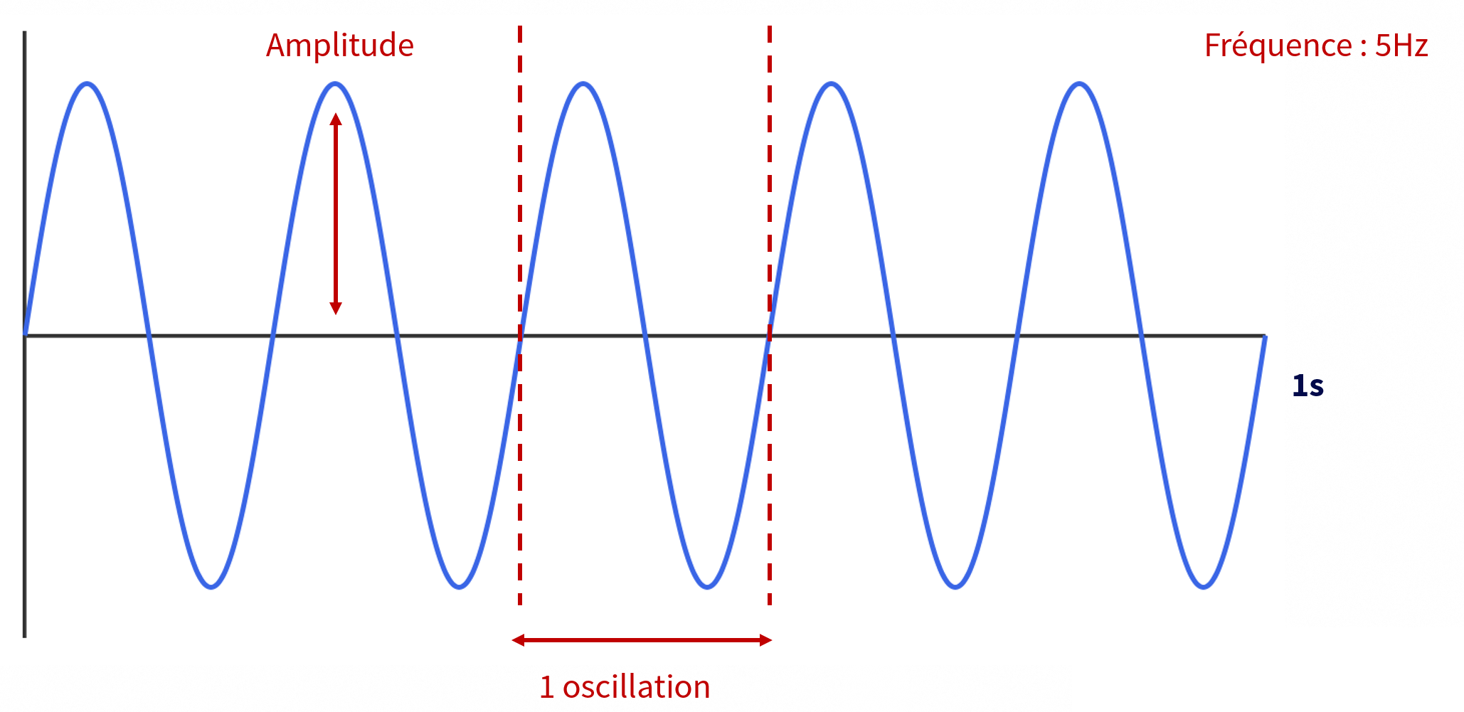
When a sound contains only a single sinusoidal frequency, it’s called a pure tone. This is precisely what ringing-type tinnitus sounds like.
It’s also the kind of sound you hear when you strike a tuning fork, or when you listen to the dial tone of a phone while trying to call someone (in France, it’s also the same continuous sound you hear on landline phones). These sounds actually share the same frequency: it’s the note A (more precisely A4 in international notation, i.e. La3 in French notation). The frequency of this A was historically set at 440 Hz in 1939 for worldwide standardization purposes, and it’s now used as the default reference frequency for tuning instruments and studying sound.

As humans, we’re able to perceive sounds whose frequency lies between 20 Hz and 20,000 Hz (20 kHz).
Below 20 Hz, we’re talking about infrasound, and above 20 kHz, about ultrasound. These sounds are not audible to humans.

Okay, now this is starting to make a bit more sense to me, but what I’m interested in is how to produce sound with a computer.
To produce / store an image, I get it: you take colored pixels, you put a lot of them in a matrix, and that makes an image.
But for sound, how does it work?

Sampling

It was by asking myself this question that I started to grapple with sampling. It’s the absolute foundation of all sound production in computing.
In reality, sampling wasn’t born with modern computing. It’s a fundamental principle of signal processing that has been used in physics for a very long time. The goal is to transform a continuous phenomenon (one that evolves without interruption, like temperature, wind or sound) into a series of discrete values (isolated numbers).
The reason is simple: we can’t store infinity in memory. So we chop it up in order to record it, analyze it and manipulate it (here, that’ll be in our code).

Sampling consists in recording the amplitude of the sound wave at extremely short and regular time intervals. The computer will note the pressure value at each instant T, and it will do so thousands of times per second.

Take cinema. In real life, motion is continuous. But a camera simply captures 24 frames per second to recreate it on a screen.
For sound, it’s exactly the same logic, we just go much faster.

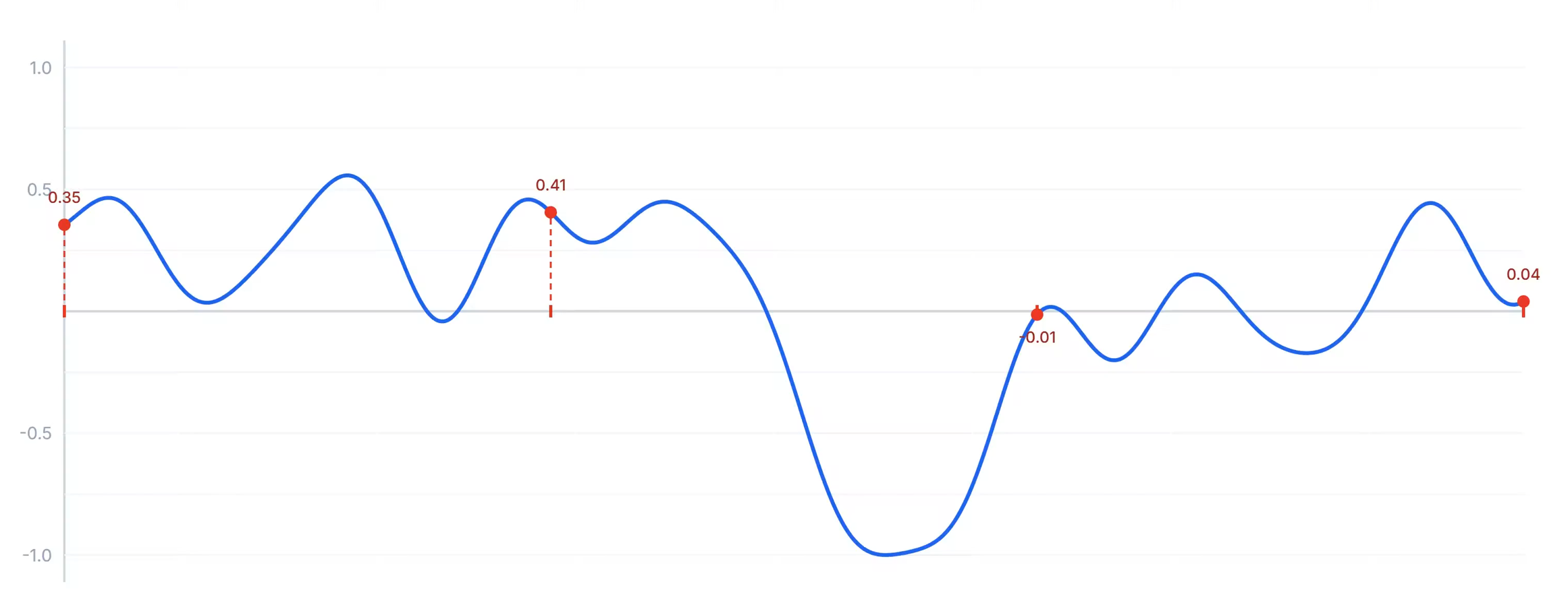
In this example, we record the amplitude 4 times at regular intervals along the signal. That’s 4 pieces of information taken directly from the signal, and they’re digital: it means we’ll be able to store and process them with a computer.
The thing is, 4 pieces of information is far too few to do anything with. The idea will then be to increase the sampling rate until we can faithfully reproduce the signal, using nothing but digital values.

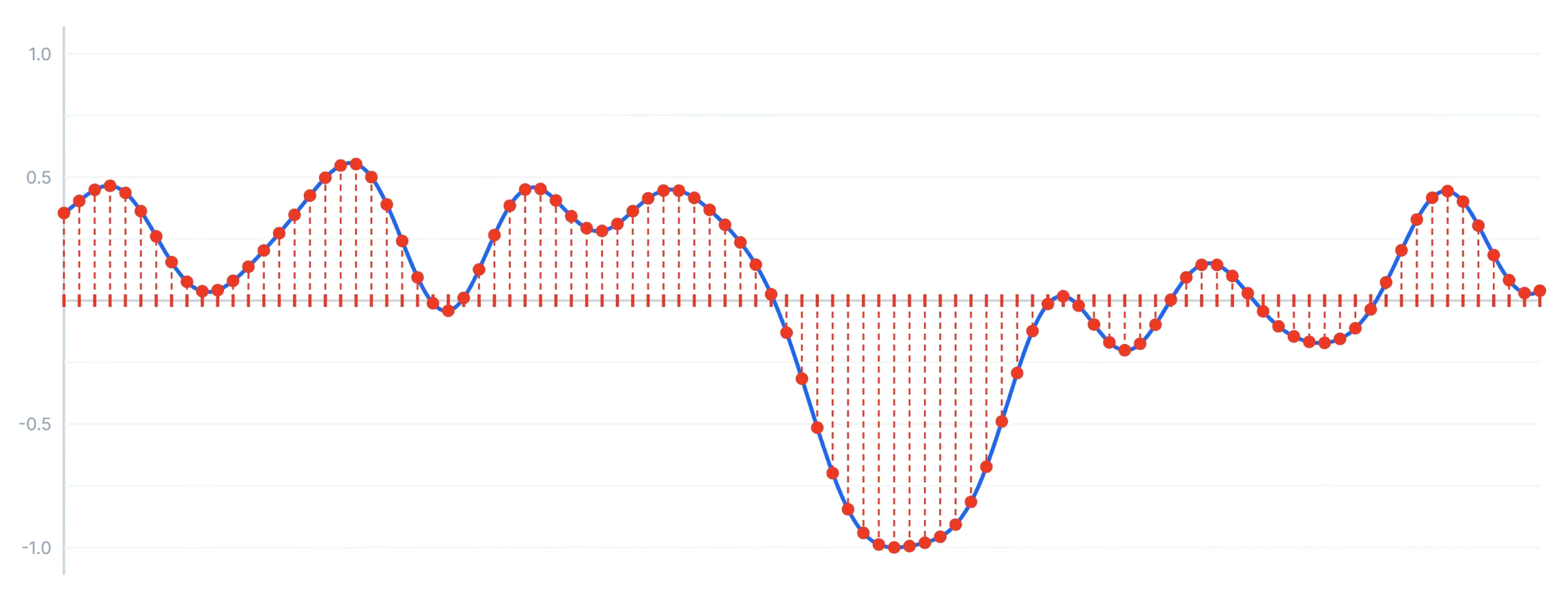
Much better!
A question then arises: we’re not going to record an infinite number of amplitudes, so how many samples per second should we record for the signal we want to create?

If we take the example of a standard audio file, we use a sampling rate of 44,100 Hz. This means that for every second of sound, the computer records exactly 44,100 mathematical values representing the air pressure. Put end to end and played back at the right speed, this data recreates the continuous sound wave for our ear.

There are several reasons behind this choice of sampling rate. The reason for the chosen order of magnitude is very important: as said before, the human ear can only perceive sounds whose frequency lies between 20 Hz and 20,000 Hz.

According to the sampling theorem (or Nyquist-Shannon theorem), in order to correctly digitize a continuous signal without loss or distortion, you have to sample at at least twice its highest frequency.

Since the highest frequency audible to humans is 20,000 Hz, we’ll then need to sample our signal at at least 40,000 Hz. This value was later raised to 44,100 Hz for the audio CD, first to leave some headroom for the anti-aliasing filter, and then because this exact figure came from the hardware of the time: digital audio was then stored on video tape recorders, and 44,100 Hz was the rate compatible with both PAL and NTSC video formats.

We finally have the basic knowledge we need to generate our white noise, it’s time to get to the code!

Let’s generate our first white noise

Setup

First step, choosing a programming language.
After some research, I went with C++, using the JUCE framework.
I chose to use a technology designed for developing highly advanced and complex audio tools, just to play around with noises. Yes, it’s totally overkill, but I wanted to have fun and discover something new.
Here, I don’t intend to develop any software whatsoever, just to generate sounds with some of JUCE’s features.

I designed my code so as to have:

Small sound generators.
A runner, which takes one of these generators as a parameter to actually create the audio file.

The idea is to factor the code as much as possible, so that the different algorithms I’ll be writing can be neatly split into files.
In short, the sound generator does nothing but fill a buffer of samples. It contains a single function: fillBuffer, which describes an algorithm for building a sampling.
The runner, for its part, takes the sampling and produces the sound file.

Once this architecture is in place, I can focus on writing the sampling algorithms.
I won’t dwell on how this implementation works since that’s not what we’re interested in here. The full source code will be provided further down.

Let’s generate white noise

Now the fun begins!
We have the basic knowledge and tools needed to create our white noise. What we’re missing now is a definition. What is white noise?

Wikipedia definition: White noise is a realization of a random process in which the power spectral density is the same for all frequencies of the bandwidth.

This definition may seem complex to you, especially because of the notion of power spectral density. It will become much clearer once we start visualizing what we’re doing. In the meantime, I suggest we focus on the random part of this definition.

Basically, it means that on average, we’ll hear all frequencies “at the same time” in the audio file.
When I talked about sound signals earlier, I showed a pure tone, with a single frequency.
The sounds we hear every day are made up of a multitude of frequencies.
That’s right! And the best part is that it’s even fairly easy to clearly break down the frequencies that make up a sound, thanks to a well-known mathematical tool: the Fourier transform.

Fourier transform

And this can be demonstrated thanks to the famous Fourier transform.

The famous mathematician Joseph Fourier formulated the Fourier integral in 1811, which gave birth to the Fourier transform.

Wikipedia definition: The Fourier transform represents a function by the spectral density it comes from, as an average of trigonometric functions of all frequencies.

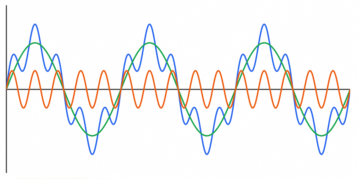
This means that any signal (here, an acoustic one) can be broken down into a multitude of sine waves. Frequencies, in other words. Take for example this relatively simple signal:

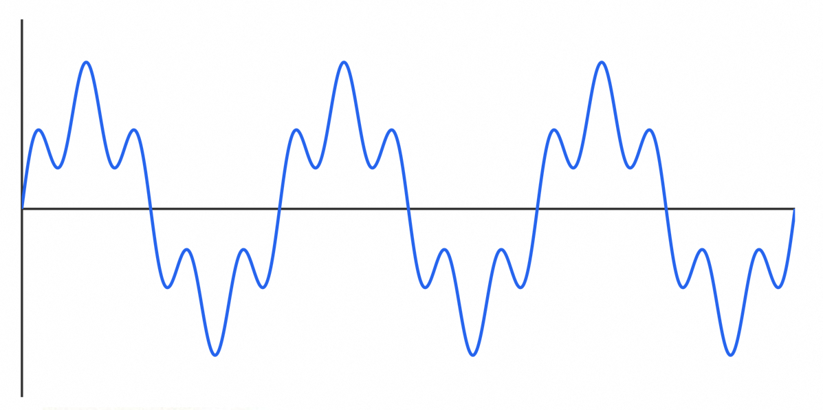
Although simple, this signal isn’t a sine wave. This means that with the Fourier transform, we can break it down into a sum of sine waves. Here, this signal is made up of two sine waves:

Back to our white noise

You may be wondering right now what this mathematical aside has to do with the definition of white noise. I said just before that white noise was a noise containing, on average, “all frequencies” over a given period of time.
The signal of a white noise looks like this:

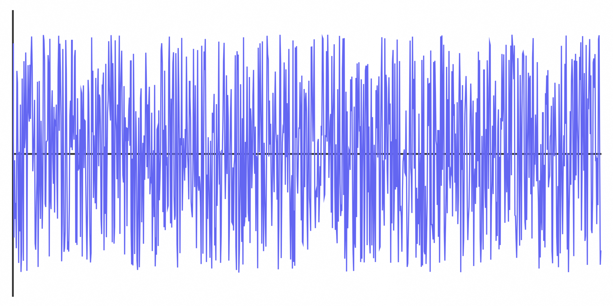
This way of representing a wave is called an oscillogram. This representation is used to visualize the shape of the wave.
Here, it’s completely chaotic.

White noise is quite simply the most chaotic noise there is. It’s totally random. What I mean by that is that to build it, all you need to do is produce a sampling by assigning a random value to each of the samples that make it up.

The algorithm will therefore be very simple:

 1
 2
 3
 4
 5
 6
 7
 8
 9
10
11
12


void WhiteNoise::fillBuffer(juce::AudioBuffer<float>& buffer) {
    const int numChannels = buffer.getNumChannels();
    const int numSamples = buffer.getNumSamples();

    for (int ch = 0; ch < numChannels; ++ch) {
        float* data = buffer.getWritePointer(ch);

        for (int i = 0; i < numSamples; ++i) {
            data[i] = random.nextFloat() * 2.0f * amplitude - amplitude; // amplitude = 1.0f
        }
    }
}

Let’s break it down simply:

numChannels describes the number of channels. 1 for mono sound, 2 for stereo sound. So we’ll make sure to write to every channel.
numSamples describes the number of samples per audio channel. It’s computed upstream by multiplying the sampling rate (44,100 Hz) by the duration.

Then, we’re going to write amplitude values “by hand”, sample by sample, until the entire sampling is filled.
Trying to produce music this way would make absolutely no sense, but to generate noise that boils down to a simple algorithm, this method is perfectly suitable.

With what we’ve just explained, the core of the algorithm that picks the value of each sample fits on a single line of code:

1

data[i] = random.nextFloat() * 2.0f * amplitude - amplitude; // amplitude = 1.0f

And that’s it.
We generate a random floating-point number between the maximum negative and positive amplitude values.
Here, we’re therefore filling our sampling with amplitude values between -1 and 1.

This will result in a totally random signal, which perfectly matches the definition of white noise.

Note: Notice that we’re talking here about “pure” randomness (pseudo-random in practice, but that changes nothing here), with values that are decorrelated from one another. No value influences the next.

One may then ask: why does a totally random variation of amplitude give us a noise that statistically contains all frequencies?
Quite simply because the frequency of a wave is directly correlated to its amplitude variations.

Take the following diagram:

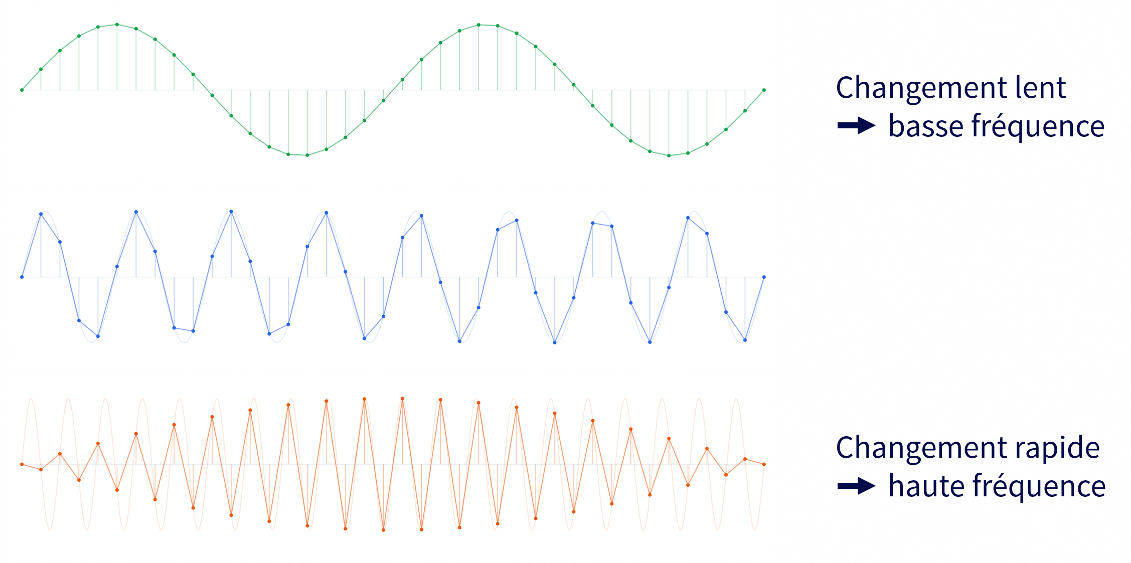
On the same time scale, describing a slow amplitude variation will allow us to reproduce a low-frequency signal.
Conversely, a fast amplitude variation will allow us to reproduce a high-frequency signal.

It then becomes clearer that a strictly random amplitude variation at each sample of our sampling will give us both low and high frequencies.

It turns out that by creating a noise from such a signal, if we broke it down with the Fourier transform, we would statistically find all the frequencies of the bandwidth at roughly equal power density.
That’s the whole magic of white noise: mathematically, a totally unpredictable and decorrelated signal (where each sample is chosen at random with no connection to the previous one) has a constant power spectral density.

By applying the Fourier transform to this signal, we notice that the energy is spread perfectly evenly across the whole spectrum, from sub-bass to ultrasound. Since no frequency is favored by chance, they are all present at the same level “on average”. It’s precisely this frequency “equality” that defines white noise.

By filling our buffer with pure randomness, we have therefore generated a signal that statistically contains every frequency of the audible spectrum simultaneously.
White noise, in other words.

Let’s listen

It’s time to listen to our white noise!

Turn the volume down if you’re wearing headphones, it can be loud and harsh on the ears.

Sound description: a big, fairly aggressive PSSSSSSCCCCHHHTT reminiscent of the sound emitted by old CRT TVs.

Ah.
We’re a long way from the relaxing sound we were looking for. You now understand why I told you that the sound you listened to earlier wasn’t really white noise, but rather one of its variants.
Where did I go wrong? Why doesn’t it sound anything like the video I found on the internet?

The answer is that I didn’t get my implementation wrong. The definition of white noise is very simple, as we’ve seen, there was little chance of me getting that wrong.

My mistake comes from my misunderstanding of the human brain, and of the way we perceive frequencies.

Our ear doesn’t perceive sound linearly: we don’t perceive all frequencies the same way.
Our perception of sound is logarithmic.
It’s clearer if I show you this table of octaves:

Band (octave)	Computed frequency
0	31.25 Hz
1	62.5 Hz
2	125 Hz
3	250 Hz
4	500 Hz
5	1,000 Hz
6	2,000 Hz
7	4,000 Hz
8	8,000 Hz
9	16,000 Hz

We can see that there’s about 30 Hz of difference between the first two octaves, and 8,000 Hz of difference between the last two.

This means that it’s far better at grasping differences between low frequencies than between high frequencies. Moving up an octave amounts to doubling the frequency.
For our ear, going from 100 Hz to 200 Hz is a major event (an octave). Going from 10,000 Hz to 10,100 Hz, on the other hand, is almost imperceptible. Yet on a linear graph, these two 100 Hz gaps take up the same space.
Hence the counter-intuitive side of white noise.

One of the consequences is that we’ll perceive high-pitched sounds more, which are unpleasant and aggressive to the ear, because each high octave physically contains many more frequencies (and therefore more energy) than a low octave. For our ear, it’s an overload: where a low octave only spans a few dozen hertz, a high octave throws thousands at it. It’s this massive density of information that creates this feeling of aggression and unpleasant hissing.

What’s interesting about this problem is that you only need to understand it to glimpse the solution.
But before tackling this solution, I think it’s high time we started putting visuals on these noises we’re talking about.

Good thing we’ve covered the principle of the Fourier transform, because I can now introduce you to a tool that relies heavily on it: the spectrogram.

Even more visual: spectrograms

The idea of a spectrogram is to visualize all frequencies on a spectrum. It’s a kind of chart where the Y axis represents frequencies (high ones at the top, low ones at the bottom), the X axis represents time, and the color expresses the power of the sound signal.
Power is defined by the intensity of each frequency over the given short period. We can therefore easily visualize the dominant frequencies of the sound in real time.

Let’s try with an excerpt from a pop rock song: Miracle by Tip Stevens.

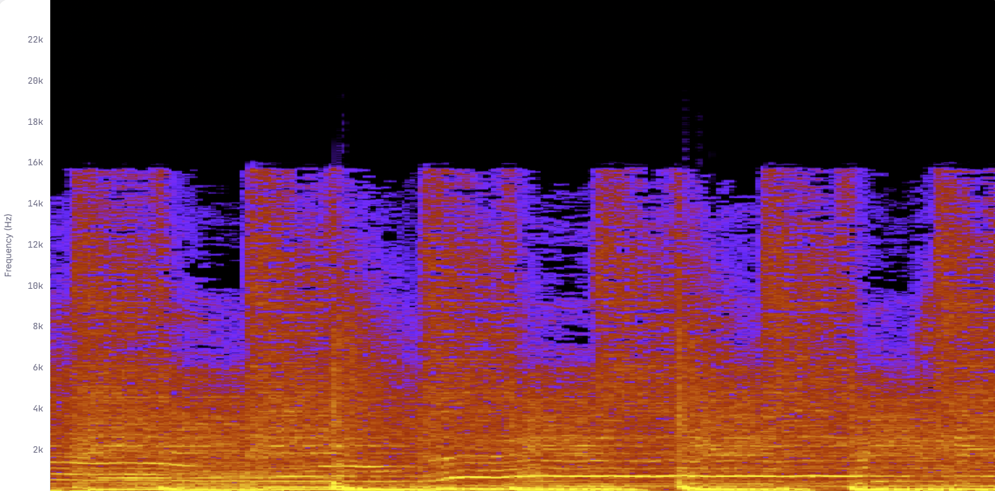
Something’s off with this visual. It’s factual regarding the frequencies present in the audio file, and yet, I have a hard time agreeing with what I see. All the frequencies seem squashed toward the bottom.

We therefore need to apply that same logarithmic scale to the spectrogram if we want a visual that matches what we actually hear:

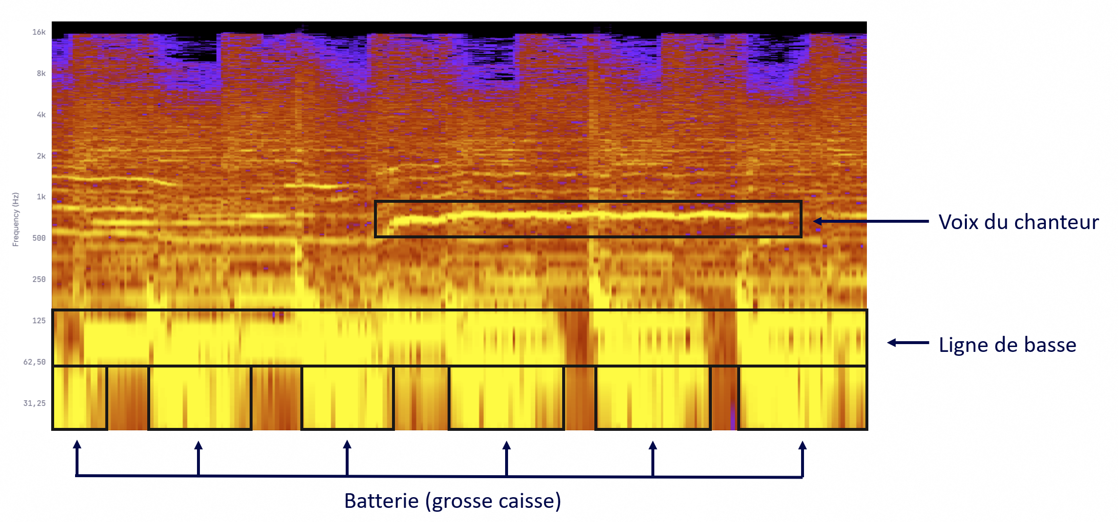
This is what’s called logarithmic scaling.

Now that’s more telling! If we listen to the song while watching the spectrogram scroll by, we can clearly see the frequencies occupied by each instrument.

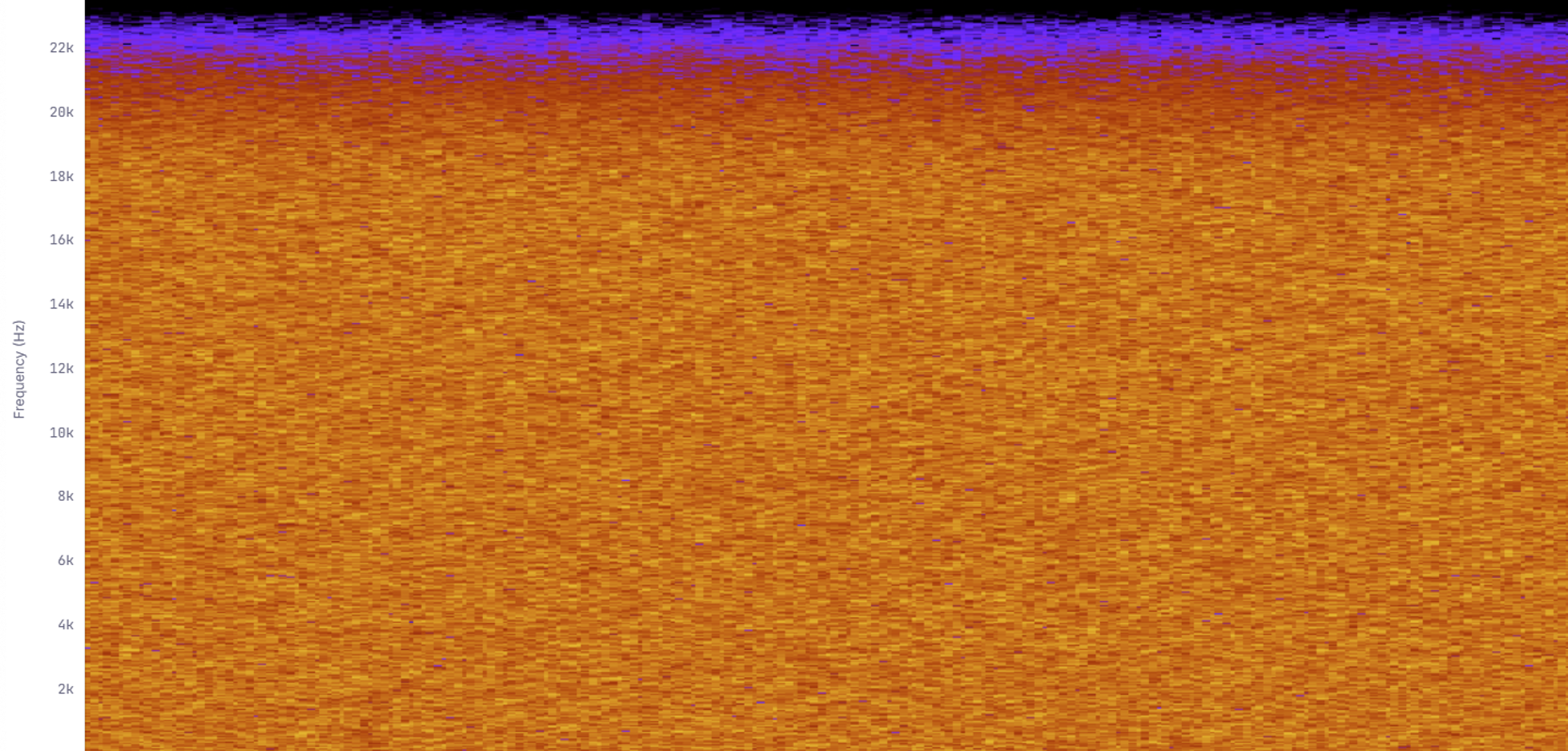
Now that we’ve seen what a song looks like, what if we tried to visualize our white noise?

Without scaling:

With logarithmic scaling:

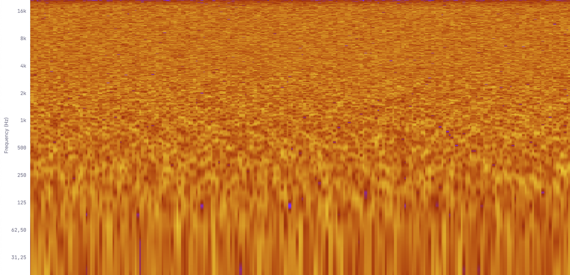
What was demonstrated by the Fourier transform above is now even more visual: with our sound generated from random amplitudes for each sample, we can clearly see here that, statistically, all frequencies are represented in roughly equal proportions across the spectrum.

Thanks to this scale, we can easily see the octaves. If we draw lines, we visually find our problem again:

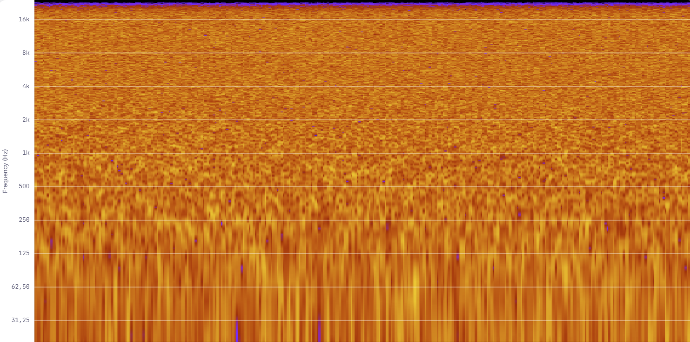
We can clearly see that for each octave band, we have twice the frequency density compared to the previous one.

We can then glimpse the solution: a variant of white noise, for which the power spectral density stays constant per octave band.
This noise would then be like white noise, but adapted to our acoustic perception, since we would truly perceive as many high frequencies as low ones, and we could get that neutral noise we’re looking for.
This noise has a name: pink noise.

Pink noise

Principle of pink noise

Wikipedia definition: Pink noise is a random signal whose spectral density is constant per octave band. Its power spectral density is inversely proportional to the frequency of the signal.

Put more simply: every time the frequency doubles, the power per hertz is halved. This is what we write as 1/f: power decreases as the inverse of frequency. And as we saw above, an octave contains twice as many hertz as the previous one. Twice as many frequencies, each half as powerful: that makes the same energy per octave. The two sentences of the definition therefore say the same thing.

There’s an algorithm specifically designed to generate pink noise: the Voss-McCartney algorithm.

Voss-McCartney algorithm

The Voss-McCartney algorithm is a very efficient method for producing pink noise (more precisely, a very good approximation of this 1/f decay). The principle is to mix several independent white noise sources, but with a twist: they don’t all “move” at the same speed.

The sources that create the high-pitched sounds change value all the time (very fast).
The sources that create the low-pitched sounds change value much less often. By adding all this up, we get a near-perfect balance that mimics our perception: each octave receives the same dose of energy.

Here’s the theoretical pseudo-code for this algorithm:

 1
 2
 3
 4
 5
 6
 7
 8
 9
10
11


n_streams = number of random streams // Number of sources
streams = [random() for _ in range(n_streams)] // We create the sources by assigning each of them a random value between 0.0 and 1.0
output = [] // Final sampling that will contain the pink noise

for i in range(total_samples): // We iterate over all samples (44,100 samples per second)
    for j in range(n_streams): // We iterate over all sources
        // Most important line: it means that each source gets refilled twice as slowly as the previous one
        if i % (2**j) == 0: // 2**j means 2^j, "2 to the power of j"
            streams[j] = random()
    // We add up all the sources to compose our pink noise
    output.append(sum(streams))

Let’s take 16 sources, which is a good compromise.
We then cover 16 octaves even though there are only 10 in the human audible spectrum, so that the 1/f decay holds all the way down to the bottom of the audible spectrum. Below the frequency at which the slowest source changes value, no source comes to reinforce the lows anymore: the spectrum becomes flat again, like that of white noise.

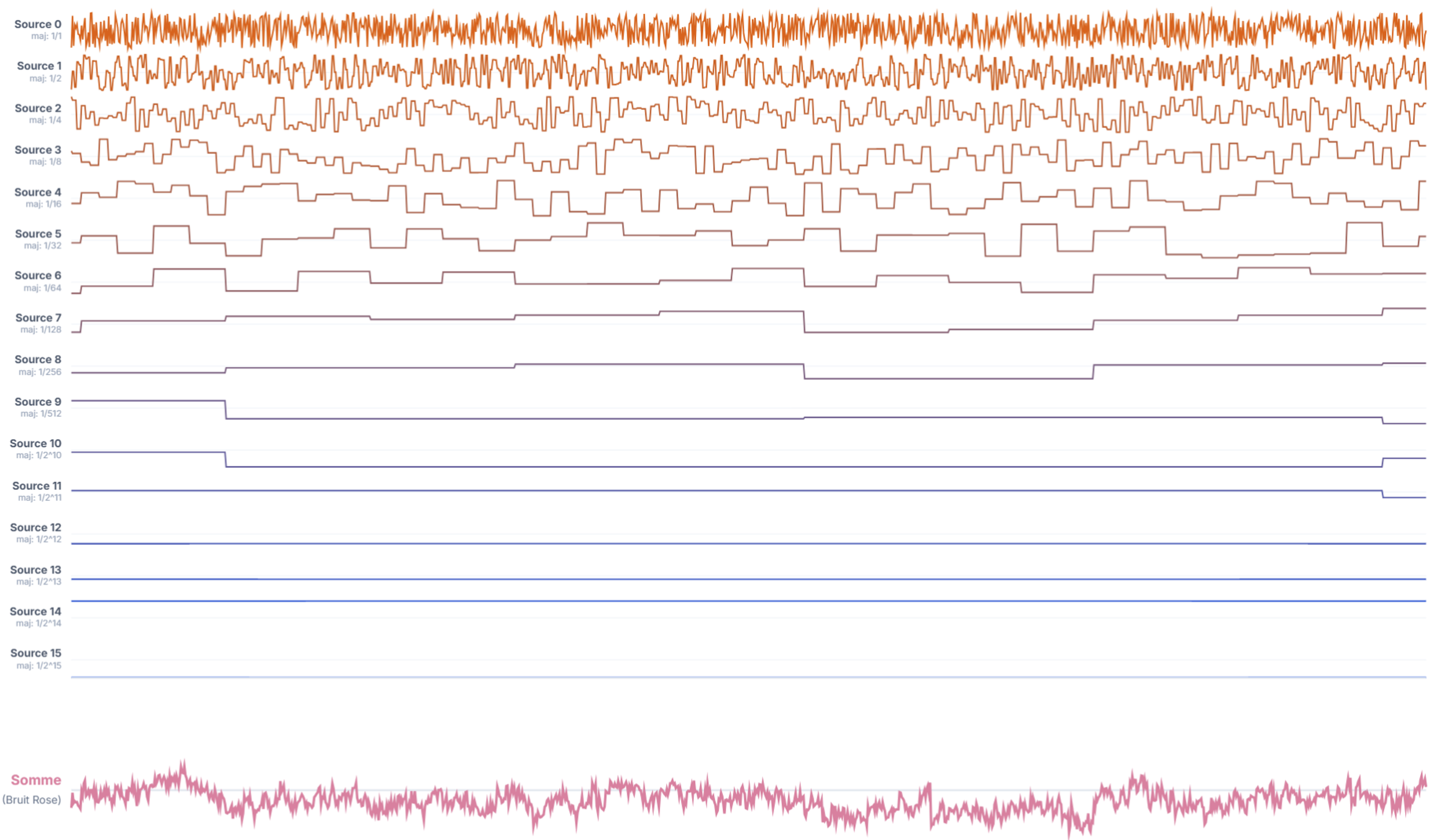
We then end up with 16 white noises, but each white noise stays “still” twice as long as the previous one.
If classic white noise contains all frequencies, as we saw earlier, from sub-bass up to 22 kHz, the next white noise, which changes value half as often over the sampling, will essentially only contain frequencies up to 11 kHz, and so on.
Each white noise source therefore contains twice as much power in the lows as the previous one.

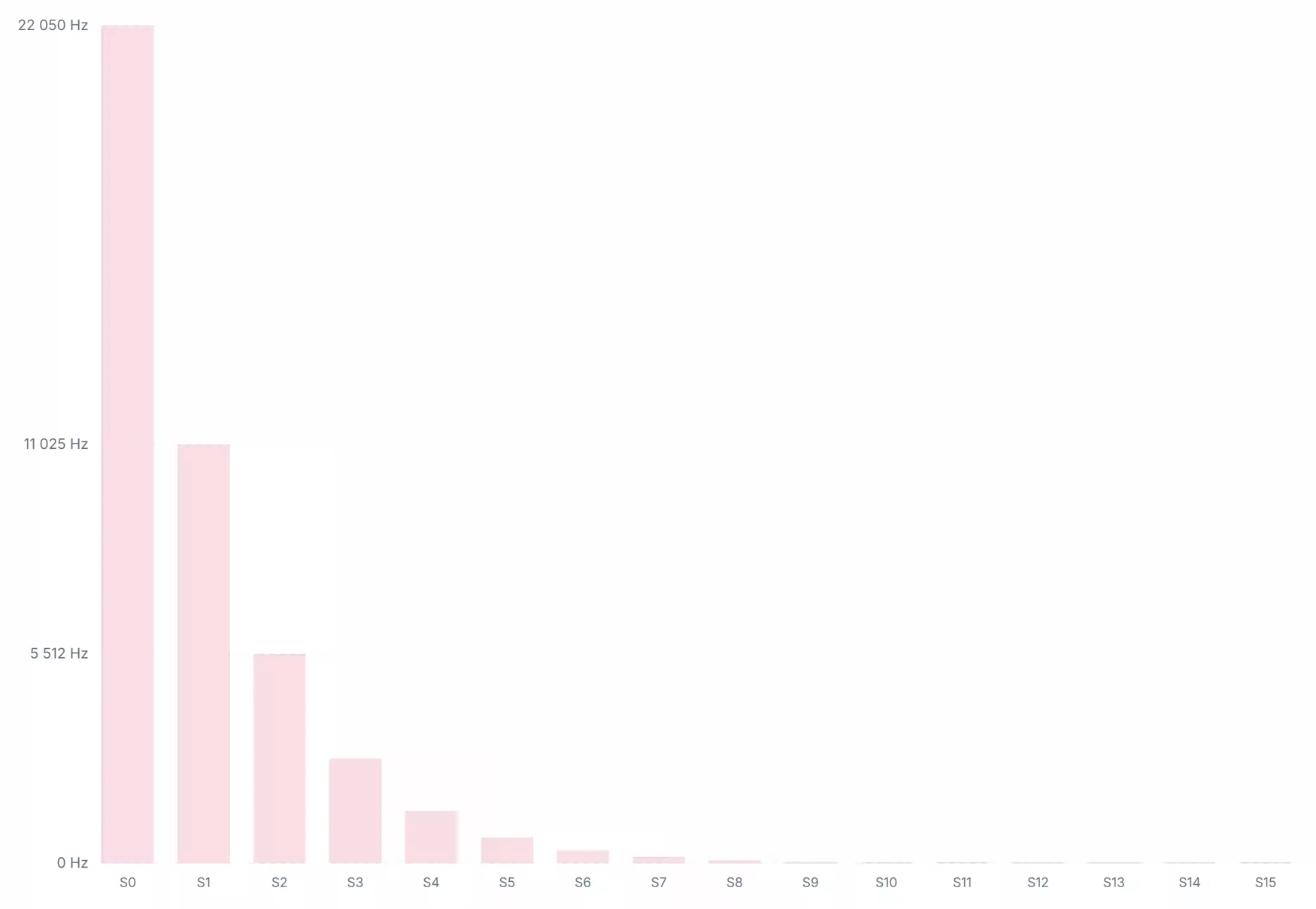
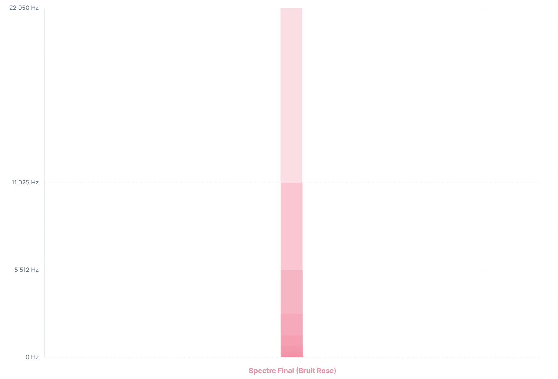
By adding up all these sources, we end up with a composition of white noises that contains more low frequencies than high ones, and this on a logarithmic scale.
Pink noise, in other words.

Here’s my implementation in C++:

 1
 2
 3
 4
 5
 6
 7
 8
 9
10
11
12
13
14
15
16
17
18
19
20
21
22
23
24
25
26
27
28
29
30
31
32
33
34
35
36
37
38
39
40
41
42
43
44
45


private:
    float amplitude;
    float softness;
    float smoothing;
    juce::Random random;

    // Voss-McCartney state
    int numRows = 16;
    std::array<float, 16> randomRows{};
    int counter = 0;
    float runningSum = 0.0f;

    // Post-filter state
    float filterState = 0.0f;

void PinkNoise::fillBuffer(juce::AudioBuffer<float>& buffer) {
    const int numChannels = buffer.getNumChannels();
    const int numSamples = buffer.getNumSamples();

    for (int ch = 0; ch < numChannels; ++ch) {
        float* data = buffer.getWritePointer(ch);
        filterState = 0.0f;

        for (int i = 0; i < numSamples; ++i) {
            int changedRow = 0;
            ++counter;
            int tmp = counter;
            while ((tmp & 1) == 0 && changedRow < numRows) {
                ++changedRow;
                tmp >>= 1;
            }

            if (changedRow < numRows) {
                float newRand = random.nextFloat() * 2.0f - 1.0f;
                runningSum -= randomRows[changedRow];
                randomRows[changedRow] = newRand;
                runningSum += newRand;
            }

            float pink = runningSum / static_cast<float>(numRows);
            
            data[i] = amplitude * pink;
        }
    }
}

And there we have it, our pink noise!

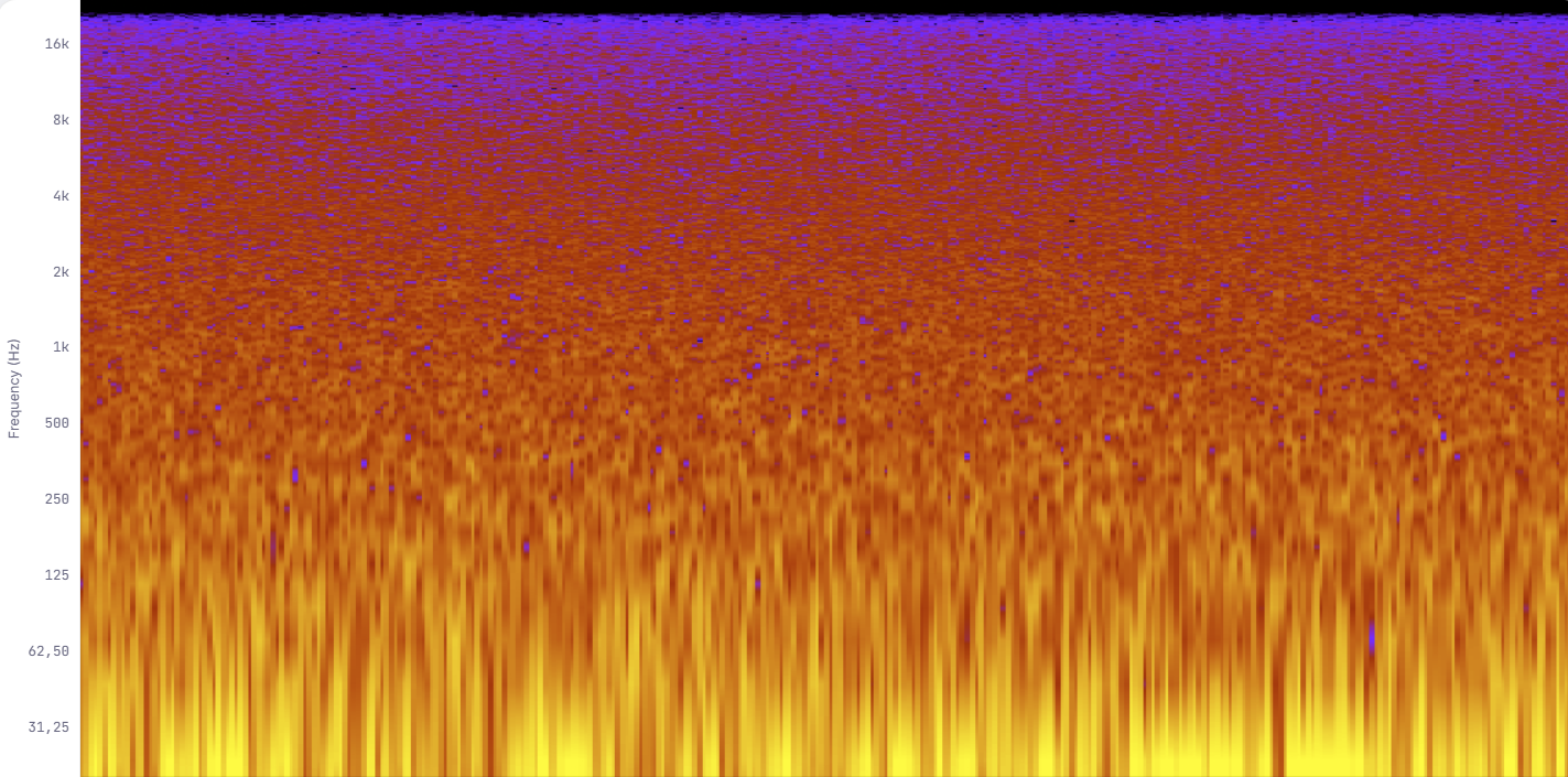
Let’s listen to it and see:

Sound description: we recognize the sound of white noise, but much softer. The noise is somewhat reminiscent of a fairly calm sea.

That’s much better, the sound is no longer aggressive, but it’s still a bit too grainy to be considered a relaxing noise.
The reason for this is first that pink noise, even a perfect one, keeps a lot of energy in the highs, precisely where our ear is most sensitive (between roughly 2 and 5 kHz). On top of that, the Voss-McCartney algorithm works the sampling values by octaves, with stair-stepped sources, as we’ve just seen.
The consequence is that we end up with abrupt jumps every time a source changes value. And remember: large amplitude jumps mean we’re generating high frequencies during these transitions.

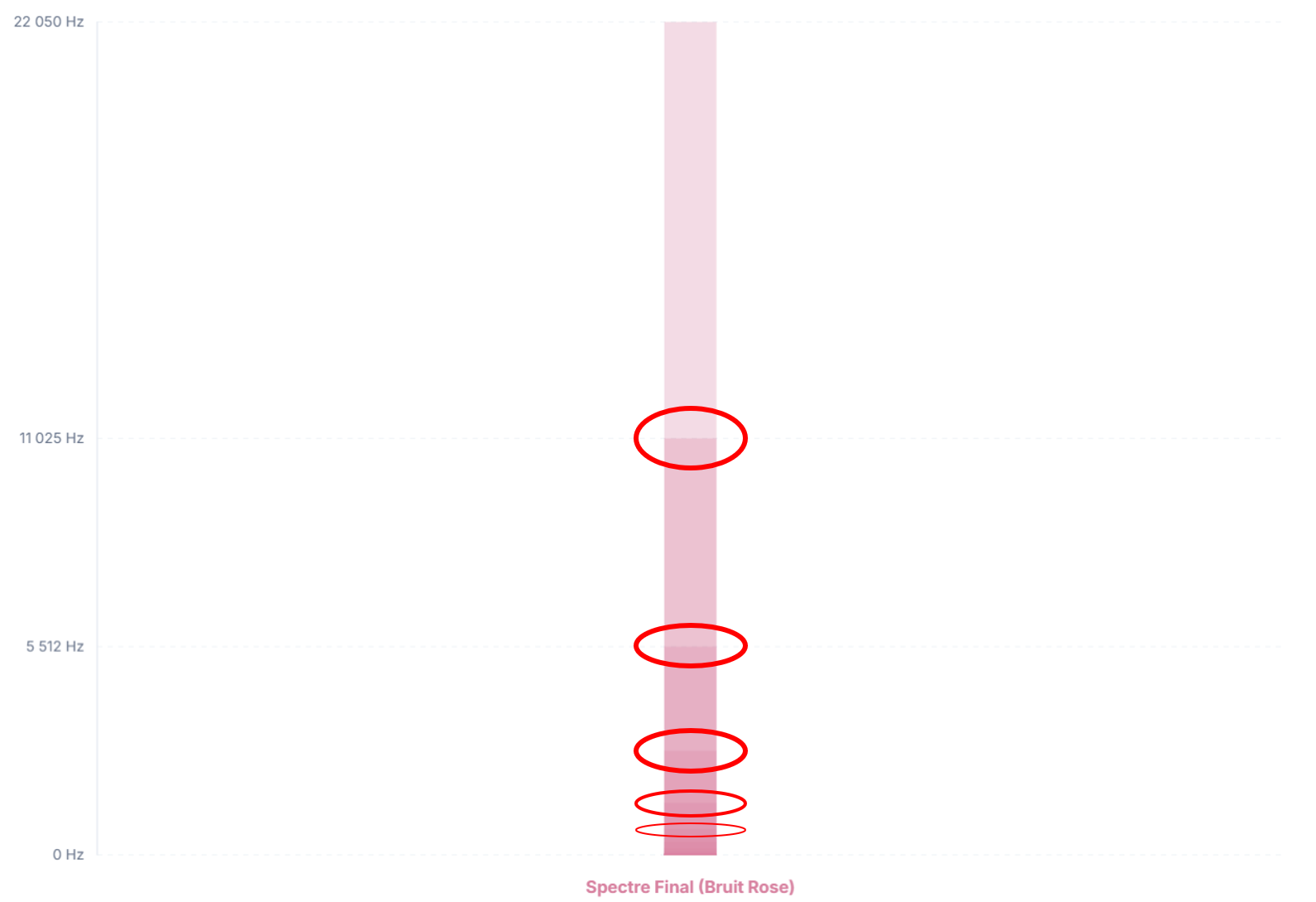
This algorithm therefore gives us almost the right solution, but we need to add a fix to it, something that will allow us to smooth out these parasitic high frequencies.
In physics, there’s a tool specifically designed to smooth out, or even eliminate, certain frequencies: filters.

FFT-based filtering

To talk about filters, there’s nothing better than introducing one of the most fascinating ones: FFT-based filtering (filtering based on the Fast Fourier Transform).

How this filter works is rather simple. We start by breaking down an acoustic signal into the different frequencies that make it up. Once that’s done, we can select the frequencies we want to eliminate, before performing an inverse Fourier transform to reconstruct the signal.
We thus get a signal similar to the original one, but with the frequencies we didn’t want removed.

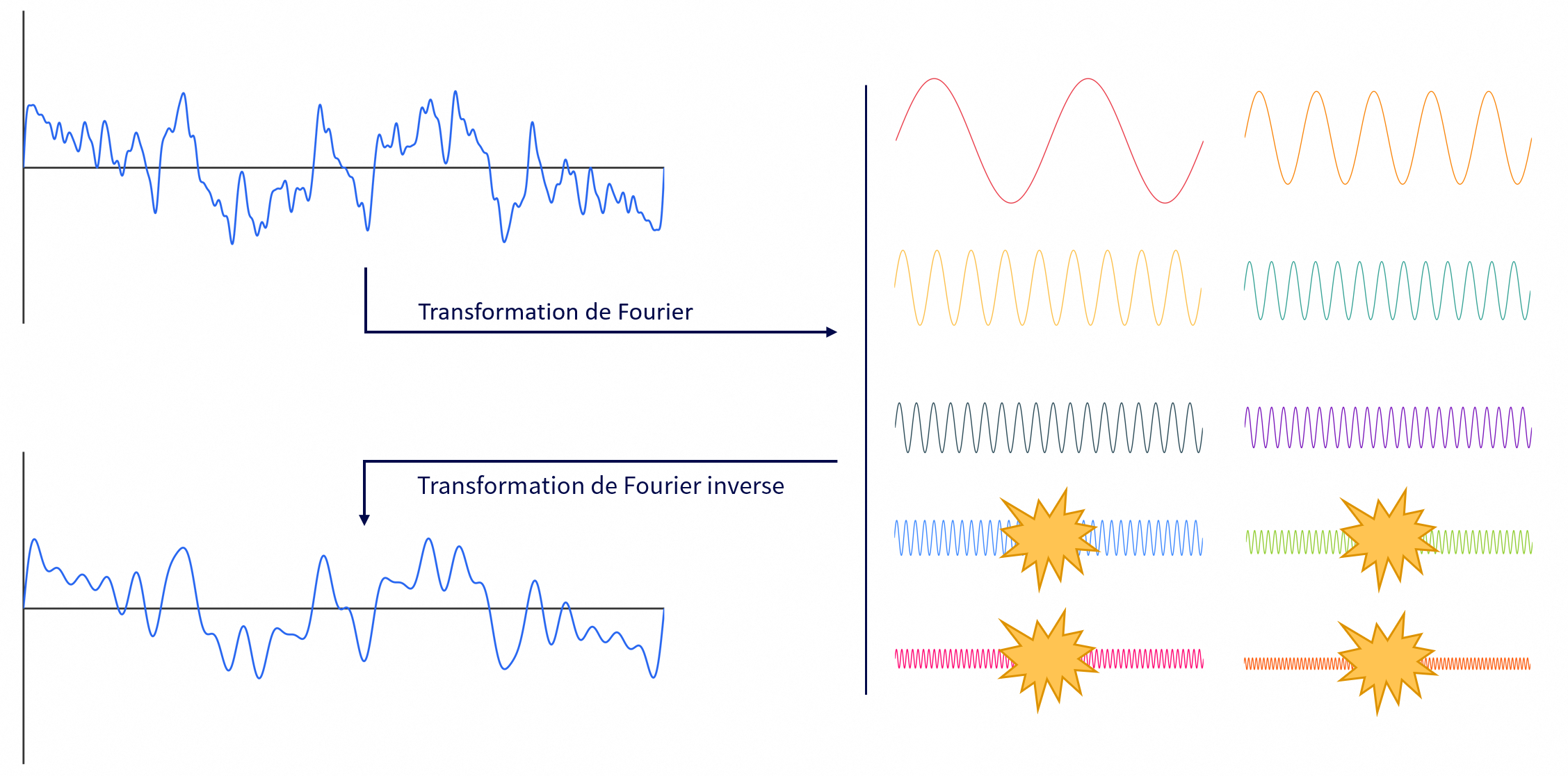
We can see in this example how to smooth a signal by eliminating high frequencies.

This is actually part of how hearing aids work, allowing them to amplify only certain frequency ranges that the patient would have difficulty hearing naturally. Hearing aids unfortunately can’t rely solely on this because of the delay induced by computation time, but it gives an idea of what this kind of filter can do: audio denoising and sound restoration, image processing and compression, telecommunications, radar, sonar, geophysics…

When you design a filter that only lets low frequencies through, it’s called a low-pass filter. In our case, we need a low-pass filter with very gradual attenuation beyond the cutoff frequency. The cutoff frequency is the threshold from which a filter starts acting: below it, the sound passes through as is, above it, it’s increasingly attenuated (by convention, it’s the point where the signal has lost 3 dB, i.e. about 30% of its amplitude). There’s a filter perfectly suited for this: the one-pole low-pass filter.

One-pole low-pass filter

A low-pass filter, in its simplest form, can be written like this:

1

filterState = smoothing * filterState + (1.0f - smoothing) * input;

That’s it. One line. And yet, it’s a filter in its own right.
It’s called a one-pole filter (or first-order IIR filter), and it’s probably the most widely used digital filter in the world.

Let’s break it down:

filterState: the filter’s current output value, i.e. the filtered sound of the previous sample. It’s the filter’s memory.
input: the raw value of the current sample.
smoothing: a coefficient between 0.0 and 1.0 that controls how “slow” the filter is to react.

The idea is simple: instead of directly using the raw value of the current sample, we compute a weighted average between the previous output and the current input.
If smoothing is close to 1, the filter “resists” fast changes a lot: the output evolves slowly, the sound becomes very soft and the highs disappear.
If smoothing is close to 0, the filter lets almost everything through: the output follows the input very closely, and the effect is almost nil.

This means that each sample becomes dependent on the signal’s history. The input value is no longer an immediate destination, but rather a direction toward which the current amplitude is pushed. By limiting the rate of change between two samples this way, we prevent abrupt changes: the signal is “braked”, which leads to a natural attenuation of high frequencies.

This filter is said to be recursive: its output depends on its own previous output. It’s precisely this feedback loop that gives it its smoothing effect. At each sample, it “remembers” a little of what it has just produced, and takes it into account to compute its next value.

The filter’s cutoff frequency (i.e. the frequency from which it starts attenuating the signal) depends directly on smoothing and on the sampling rate. The higher smoothing is, the lower this cutoff frequency, and the more damped the sound.

In my case, with smoothing = 0.8f (which gives, at 44,100 Hz, a cutoff frequency of about 1.6 kHz: below it, the noise passes through almost intact, above it, it gets softer and softer), the filter cuts enough of the pink noise’s sharpest transients without distorting the richness of the signal too much. The result is a noticeably rounder sound.

The formula is actually more readable with a defined smoothing value, such as 0.8:

1

filterState = 0.8 * previous + 0.2 * current;

It could be translated as “each new output sample keeps 80% of the previous output and only incorporates 20% of the new input”.

Here’s what a signal looks like when we apply this filter to it, with an increasingly high smoothing until it reaches 0.8:

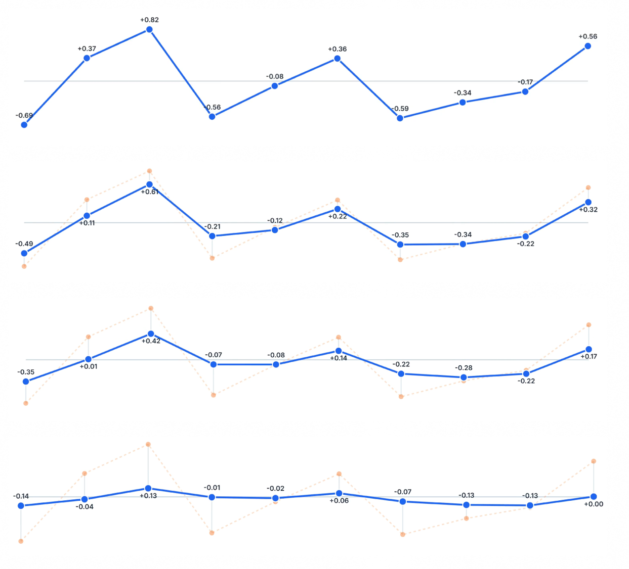
All that’s left is to apply this filter to our pink noise.

Pink noise + low-pass filter

Here’s what our pink noise looks like with a low-pass filter added:

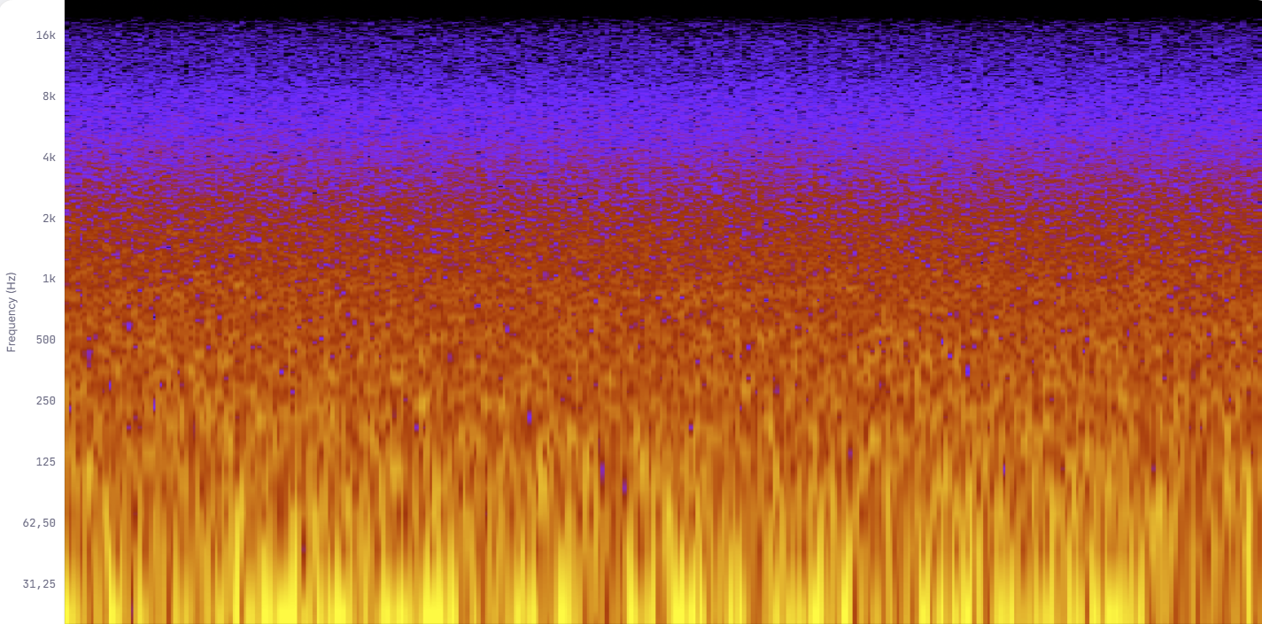
Let’s listen:

Sound description: a noise similar to a light breeze or the soft sound of a calm sea.

We finally made it! By producing our first white noise, understanding how it works, and then shaping a pink noise attenuated by a low-pass filter, we’ve achieved our goal: a perfectly functional sound to relieve tinnitus or help someone concentrate.

It’s a nice victory. There’s still so much to say in this field, but I’ll settle for introducing you to two last noises.

Other colored noises

First of all, it’s interesting to know that there’s an opposite of pink noise (which can be obtained, for example, by differentiating pink noise): a noise whose power spectral density is proportional to the frequency of the signal (rather than inversely proportional). It produces the exact opposite of what we want: a shrill noise that’s very unpleasant to the ear.
This sound is blue noise.

But also, although pink noise is one of the most used by some people for this need, there’s another very well-known noise preferred by others: red noise.

Red noise

If white noise is absolute chaos and pink noise its logarithmic balance, red noise is something deeper, lower.

Wikipedia definition: Red noise (or Brownian noise) is a signal whose power spectral density decreases as 1/f², i.e. an attenuation of 6 dB per octave. It’s the noise associated with Brownian motion.

“Brownian motion”, that sounds very much like physics. And it is indeed linked to physics: it’s the random motion of a particle subjected to perpetual collisions with the molecules of a fluid. A grain of pollen in water, for example.
But what interests us here is its audio equivalent: at every instant, the signal doesn’t head off in just any direction. It moves from where it was.

That’s exactly the logic of my implementation:

 1
 2
 3
 4
 5
 6
 7
 8
 9
10


void BrownNoise::fillBuffer(juce::AudioBuffer<float>& buffer) {
    float value = 0.0f;

    for (int i = 0; i < numSamples; ++i) {
        float white = random.nextFloat() * 2.0f - 1.0f;
        value += white * 0.02f;
        value = juce::jlimit(-1.0f, 1.0f, value); // Bounds
        data[i] = amplitude * value;
    }
}

Where white noise assigned an independent value to each sample, here we accumulate: each new value is the previous one, plus a tiny random step (white * 0.02f). The signal doesn’t jump, it drifts.
The jlimit is simply there to prevent the drift from running away and going out of bounds.

The shape of this signal is described as a “random walk”.

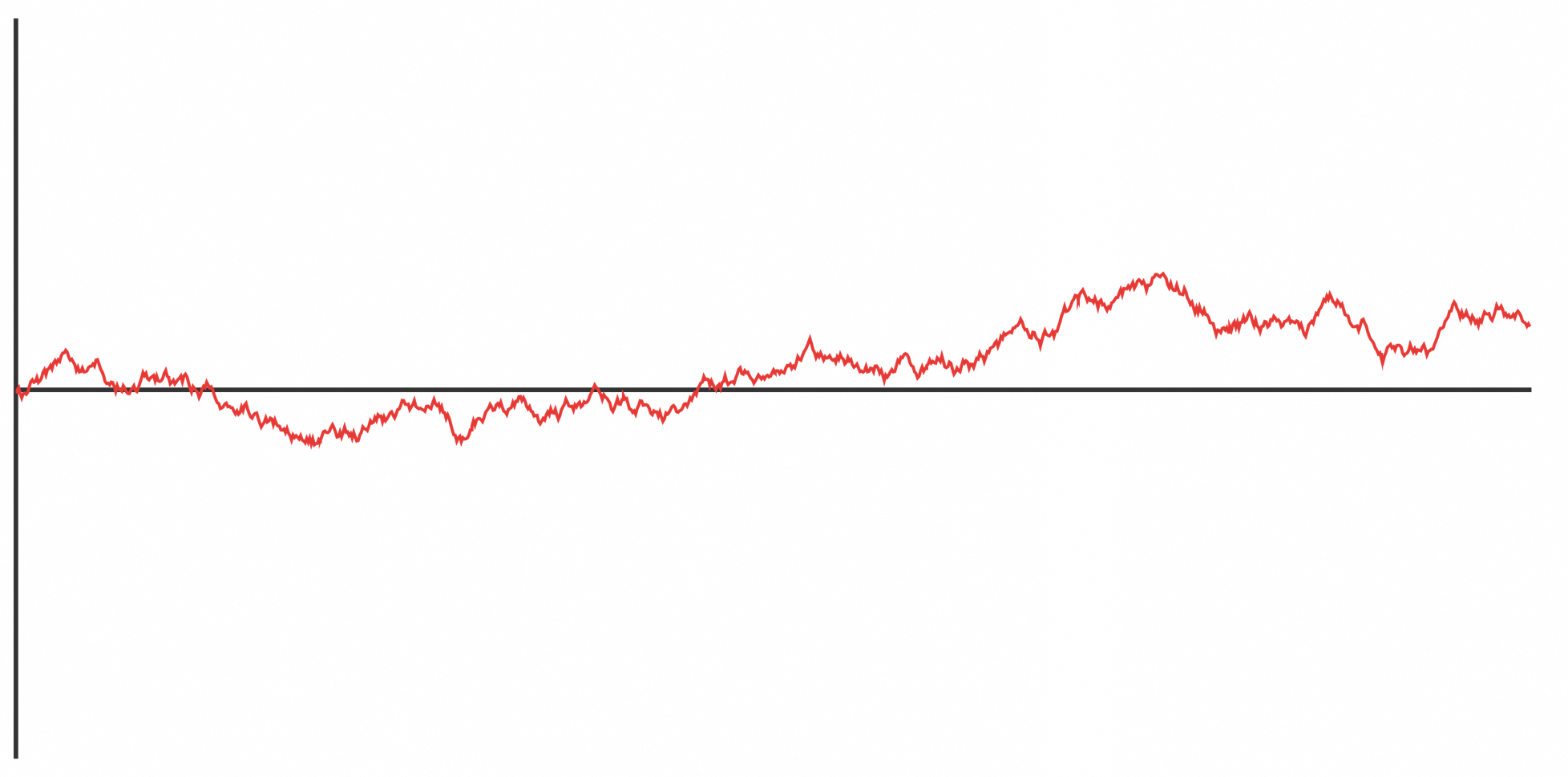
The resulting sound is something much deeper and rolling, reminiscent of distant thunder, waves, an underground river. Less aggressive than white noise, more muffled than pink noise.

Visually, on the spectrogram, the difference is immediate: where white noise carpeted the whole spectrum evenly, brown noise collapses toward the lows. The energy is very heavily concentrated in the low frequencies, and drops steadily toward the highs, at 6 dB per octave.

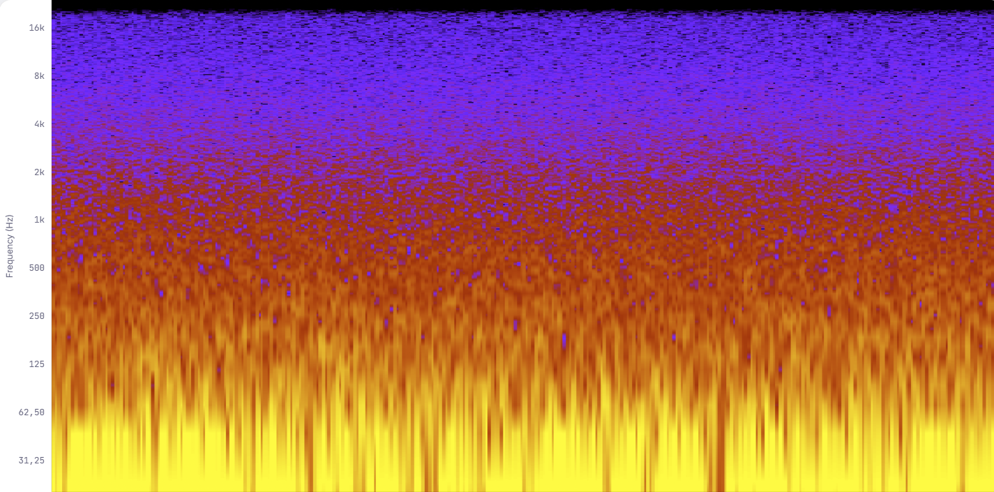
Let’s listen:

Sound description: a noise similar to a light breeze or the soft sound of a calm sea, but with a slight stormy undertone.

There are still other colored noises, such as violet, grey or velvet. A Wikipedia page is dedicated to them, feel free to check it out if you want to discover more: https://en.wikipedia.org/wiki/Colors_of_noise

We’ve reached the end of what I wanted to tell you about colored noises!
Before we part ways, I wanted to end on a fun note. When you realized that we could visualize the frequencies of a sound, didn’t you think we could use that to hide messages in a spectrogram? I did!
This process belongs to a principle called steganography.

Bonus: steganography

Steganography is the art of concealing a message within an innocuous medium, in such a way that its very presence remains imperceptible. No key, no visible encryption. The secret is that the message is there but nobody sees it (or hears it).

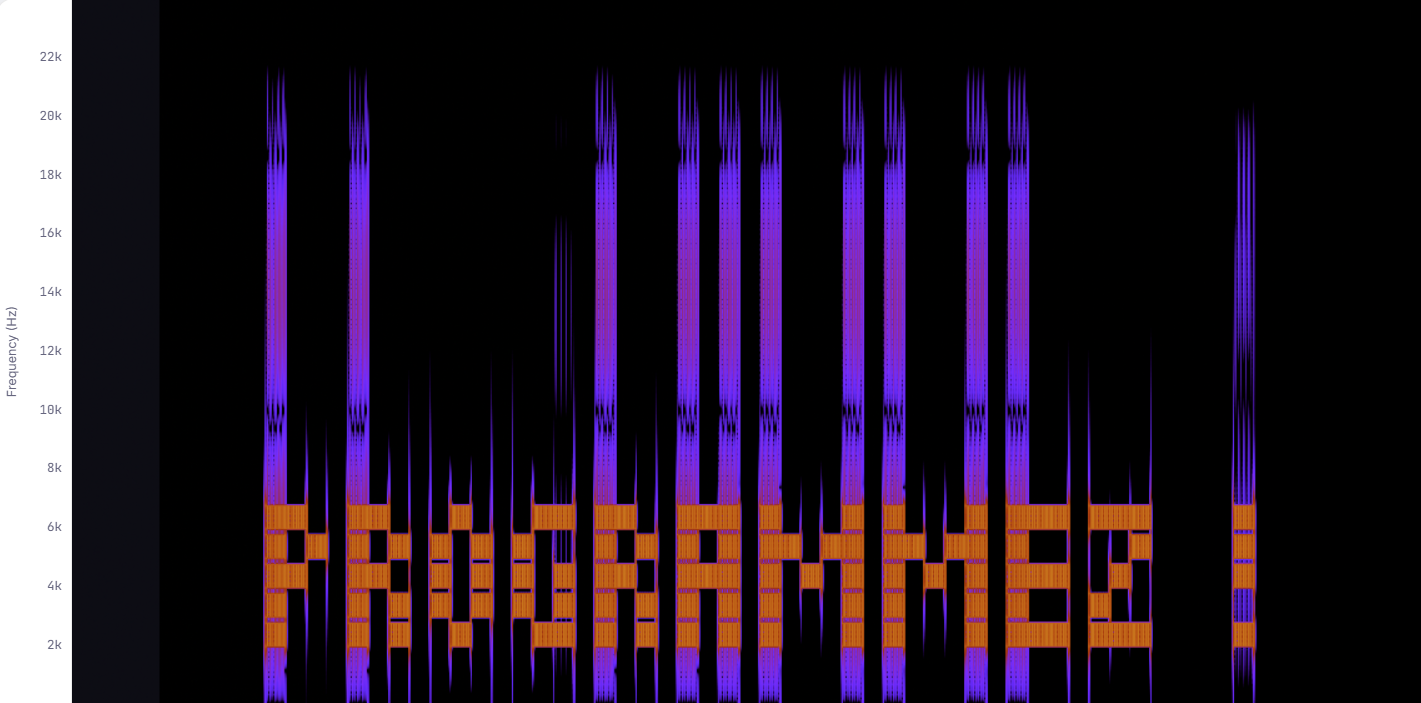
The idea here is simple: as we’ve seen, a spectrogram represents frequencies over time. If we can precisely control which frequencies are present at which moment, we can draw something in the spectrogram. And if we mix that with some background noise, the audio file remains unremarkable to the ear, but reveals its content to anyone who looks at it on a spectrogram.

The principle of my implementation: I divide the audible spectrum into frequency bands corresponding to the pixel rows of a bitmap font.
Each letter is represented by a series of 5-pixel columns. Each pixel is either on (1) or off (0).

Each band is fed by about twenty oscillators whose frequencies are spread over a range of roughly 800 Hz, which gives each “pixel” enough visual thickness to be readable on the spectrogram.

Done this way, I can get a sound whose noise sounds like an uninteresting crackle, but which reveals its message on a spectrogram:

Thank you for reading this article all the way to the end!

Talk

I had the honor of giving a talk at DevLille 2026, where you’ll find roughly the same content as in this article, told in a more narrative way.

Acknowledgements

Thanks to Tip Stevens for agreeing to let me use one of their songs for educational purposes.