Introduction to Deep Learning

Introduction

What’s in this documentation?

This documentation is an introduction to deep learning.

It’s dedicated to people who want to discover the neural networks and the world around it.

This isn’t a tutorial, this is a course whose purpose is to provide the knowledge needed to start any deep learning framework tutorial.

The purpose is to be more familiar with the neural network environment, concepts and vocabularies.

You’ll find here a description of deep learning, how to create the neural network that corresponds to your needs, and few code examples written in Python using Keras.

Keras is an open source neural network library running on top of other neural network libraries. Here, we will use Keras on top on Tensorflow.

What’s deep learning

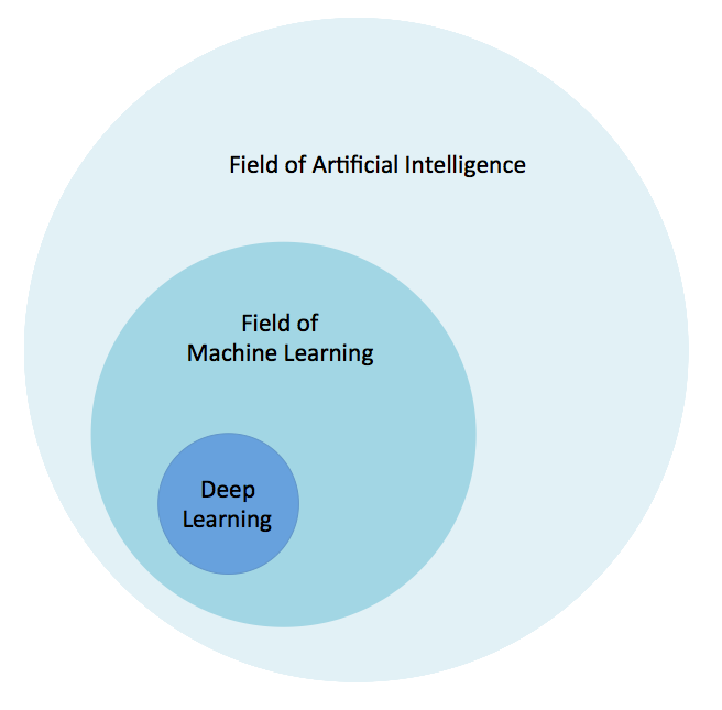
Before to talk about deep learning, let’s talk a bit about artificial intelligence and machine learning.

Personally, I would define Artificial Intelligence as the set of theories and techniques, mathematical and algorithmic implemented to simulate human intelligence.

That’s not very far from the Cambridge definition: “The study of how to produce machines that have some of the qualities that the human mind has, such as the ability to understand language, recognize pictures, solve problems, and learn”.

We can find many definitions of A.I, but all of them describe the same concept: the capability of a machine to imitate intelligent human behavior.

The purpose is to make the machine able to successfully achieve its goals as a human would do.

There are several ways to perform this approach, one of them is to allow a machine or a system to learn and improve from experience without being explicitly programmed: that’s machine learning.

Machine learning is an application of A.I.

Finally, there are some ways to do it, and one of them, a subcategory of machine learning, is inspired by the human brain and the way it thinks.

Directly inspired from the biological neural networks, the machine learning method we are going to talk about is the method using artificial neural networks. That’s what we call the Deep Learning.

Not far either from the Cambridge definition: “A type of artificial intelligence that uses algorithms (= sets of mathematical instructions or rules) based on the way the human brain operates”.

Actually, it’s quite of hard to define because it has changed decades after decades since 1980.

We can define it by a machine learning using neural networks with a large number of parameters and layers, belonging to one of the fundamentals network architectures :

Multilayers Perceptrons (MLP)
Convolutional Neural Networks (CNN)
Recurrent Neural Networks (RNN)

Historically, the first perceptron model was invented by Frank Rosenblatt in 1957, inspired by the cognitives theories of Friedrich Hayek and Donald Hebb.

That’s in 1974 that Paul Werbos proposed the first neural network model using multilayer perceptrons, then developed and perfected by David Rumelhart in 1986.

This is the first type of model we will talk about.

What can we do with it

Before to explain how it works and how to use it, it may be useful to know what need it meets.

From my experience and what I did with them, I would sum up the purpose of neural networks by “predict an output from an input, according to a training data set”. This is what we call supervised training.

Let’s explain this sentence by a simple example. You’re walking on the street, and you see a cat. The interesting thing to notice is that you obviously know that’s a cat, but you’ve never seen it before. If we were talking about an animal, or anything you’ve already seen before it would seem normal that you’re able to recognize it, but when you see something that looks like something else you already know, you don’t recognize it. You figure it out. Have you ever wondered why you are able to figure out so many thing you see every day, even though you’ve never seen them before?

The answer is simple: your brain is trained. When you see something, the picture of your sight is sent to your brain, your neural network is processing the information to guess what you’re seeing. You learn, an then you’re trained. Real biological functioning is of course much more complicated, but this explanation is sufficient to understand what the first deep learning researchers were inspired by.

We can say that the picture your brain received is the input sent to your neural network, and the guess the output.

Following this logic, if we’re able to create an artificial neural network, we would be able to recognize something it never saw before, according to a training data set you sent to it, exactly like your brain do.

It’s not hard to imagine that the possibilities are infinite.

You want to recognize hand-written letters? Build your neural network model correctly, give a huge amount of hand-written letters to it, and then try to make it able to recognize a letter it never saw before. If you built properly your model and if you have enough data for the training, you will succeed.

That’s using this method that the robots are currently able to read printed texts easily. By feeding as many fonts and handwritten letters as possible into a neural network, it will be easy to figure out text from an image.

That’s the same thing if you want to recognize faces, cars, or anything.

This method can of course be applied to any kind of data, but it’s interesting to know that today we have much better results using neural networks than classic images processing to recognize patterns in images.

If we go farther, the data prediction isn’t that far to the recognition. If I say “2, 4, 6, 8, and?”, you will answer “10”. That’s also thanks to your trained brain that you were able to figure out the following of this logical sequence.

Okay, but what’s a neural network? What it looks like? Is it easy to implement?

Multilayer Perceptrons (MLP)

Build your model: shapes recognition

Let’s start by the most classic type of model and the easier to understand, the Multilayer Perceptrons.

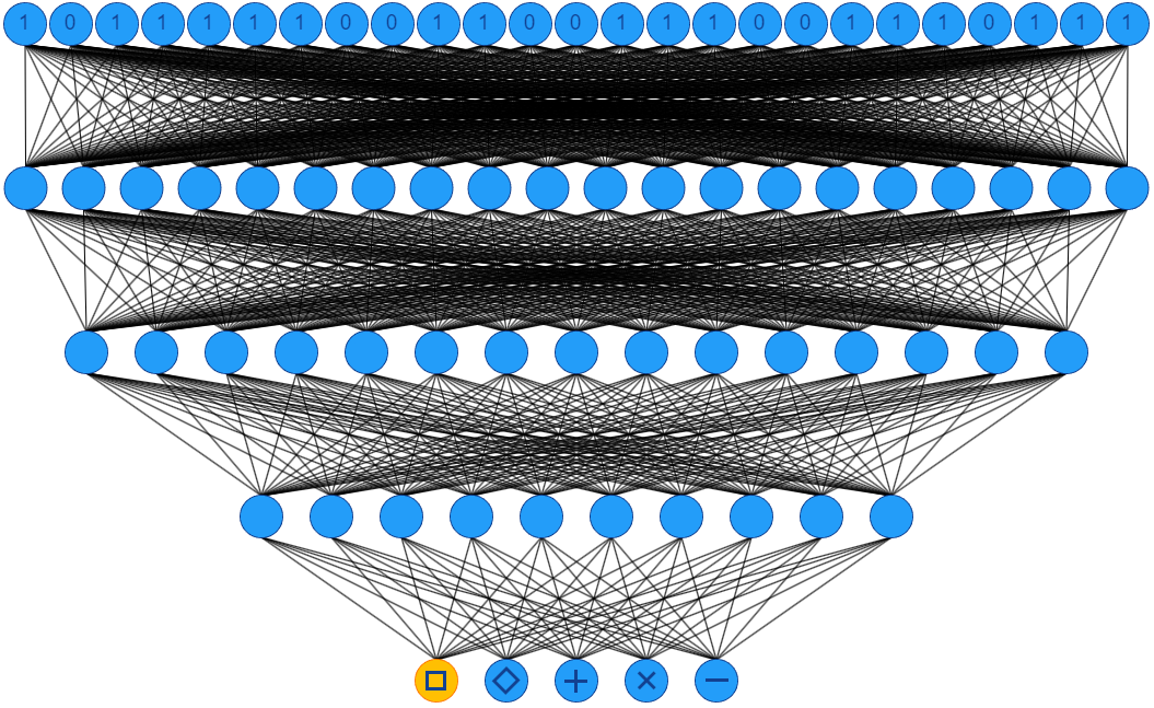
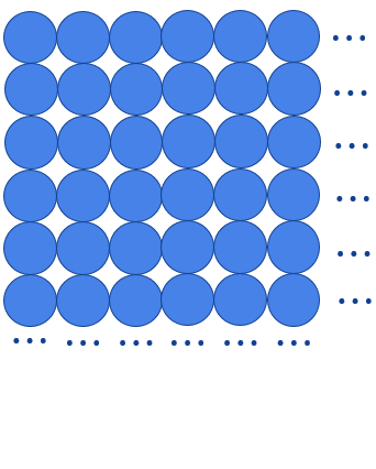
Here’s what a MLP looks like:

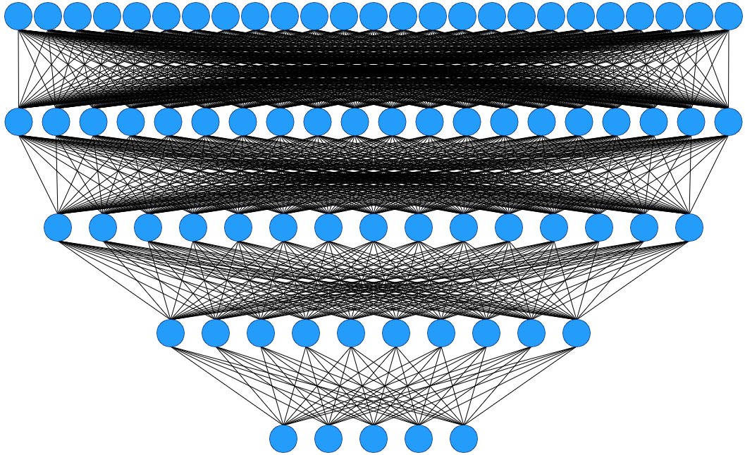
This is a 5-layers Multilayer Perceptron. It has 25 neurons in its input layer, 5 neurons in its output layer, and 3 intermediate layers. The intermediate layers are called hidden layers.

So this model is built to figure out an answer among 5 possibilities via a data that we can describe in 25 parts.

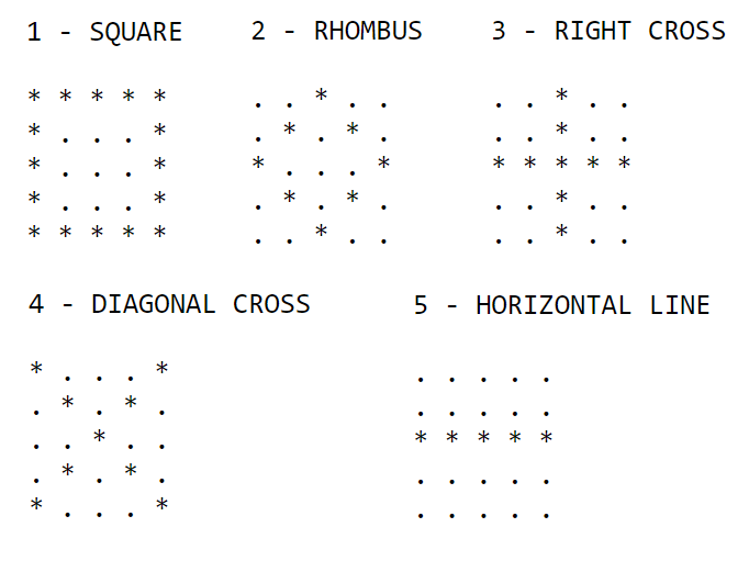
For example, we will use this model to recognize simple 5x5 shapes among 5 different shapes.

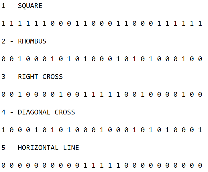
Here’s what the shapes would look like:

Build this model with Keras

 1
 2
 3
 4
 5
 6
 7
 8
 9
10
11
12
13
14
15
16


model = Sequential()
model.add(Dense(25, activation='relu', input_shape=(25,)))
model.add(Dropout(0.2))
model.add(Dense(20, activation='relu'))
model.add(Dropout(0.2))
model.add(Dense(15, activation='relu'))
model.add(Dropout(0.2))
model.add(Dense(10, activation='relu'))
model.add(Dropout(0.2))
model.add(Dense(5, activation='softmax'))

model.summary()

model.compile(loss='categorical_crossentropy',
    optimizer=SGD(lr=0.01, clipnorm=1.),
    metrics=['accuracy'])

We can see here the 5 layers declarations, with the good amount of neurons for each of them. The activation function, dropout, loss, cross entropy, optimizer and accuracy concepts will be explained in the part dedicated to the explanation how how the neural networks really work.

Now, in order to make the neural network able to recognize them later, let’s see how to use these shapes to train your model.

Train your model

Obviously, our neural network won’t understand the symbols we used to draw our shapes, we have to give to it numeric values.

If we now convert these shapes into numeric data, we have this :

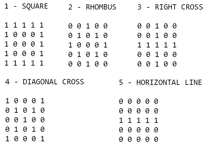
To make them fit into the neural network, we will vectorize them:

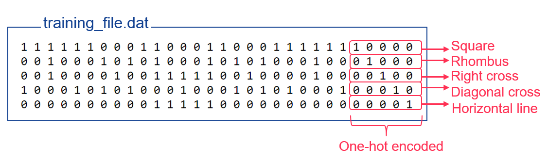
Finally, as it’s a training dataset, we have to indicate the expected result. To write it in a neural network format, we have to use the one-hot encoding.

That just means that we write 5 bits, one by possible output. The expected output for the input line is set to 1, and the others to 0. So “1 0 0 0 0” means “the first output neuron” and “0 0 0 1 0” means “he fourth output neuron”.

If you want now to write a training file with our vectorized shapes, it will look like this:

Once the neural network is trained with this dataset, if we now give to it one of our shapes like the rhombus, it will recognize it.

But it’s cheating, because this exact vector describing the rhombus had already be seen by the neural network, it belong to the training dataset, so of course the model can recognize it.

But, as you probably expect now, this trained model is now able to figure out, among shapes it never seen before, what shape does it make him think.

Train this model with Keras

1
2
3
4
5
6
7
8
9


train = pd.read_csv('training_file.dat', sep=" ", header=None)

x_train = (train.ix[:,:train.shape[1]-5-1].values).astype('float32')   #  - 5 => nb classes
labels = (train.ix[:,25:train.shape[1]-1].values).astype('int32')      #  25 => nb inputs

history = model.fit(x_train, labels,
    batch_size=1,
    epochs=20,
    verbose=1)

Test your model

Let’s try now with this broken square:

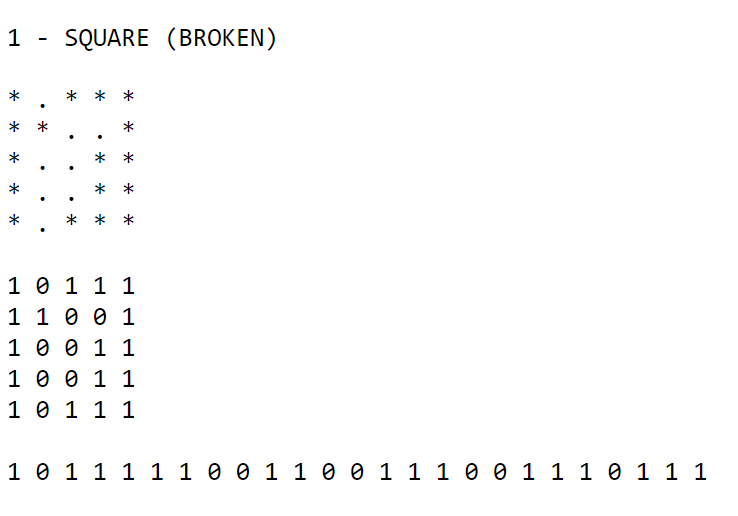
We pass the vector in the first layer:

The neural network figured it out, thanks to its training.

To be clear, this example is very simple to be as understandable as possible. The model is very light, and the training file is very weak.

We had here only one line by shape to train, for a real use case it wouldn’t be enough.

Test this model with Keras

 1
 2
 3
 4
 5
 6
 7
 8
 9
10
11


test = pd.read_csv('shapes_test.dat', sep=" ", header=None)    # shapes_test.dat => e.g: 0 0 1 0 0 0 1 0 1 0 1 0 0 0 1 0 1 0 1 0 0 0 1 0 0
x_test = (test.ix[:,:test.shape[1]-1].values).astype('float32')
outputs = model.predict(x_test)

prediction = {}
prediction['confidence'] = float(max(outputs[0]))
df = pd.DataFrame(data=outputs)
prediction['class'] = df.values[0].tolist().index(prediction['confidence'])

print(df)
print(prediction)

Output

1
2
3


0        1        2        3        4
0.016649 0.929342 0.020666 0.001302 0.032041
{'class': 1, 'confidence': 0.9293420314788818}

Character recognition

Let’s go then to a real example, which is a logical follow-up from this one: characters recognition. This use-case is more common and there are many neural network models created to do it today in production.

With the example we just talked about, it shouldn’t be hard now to understand this one:

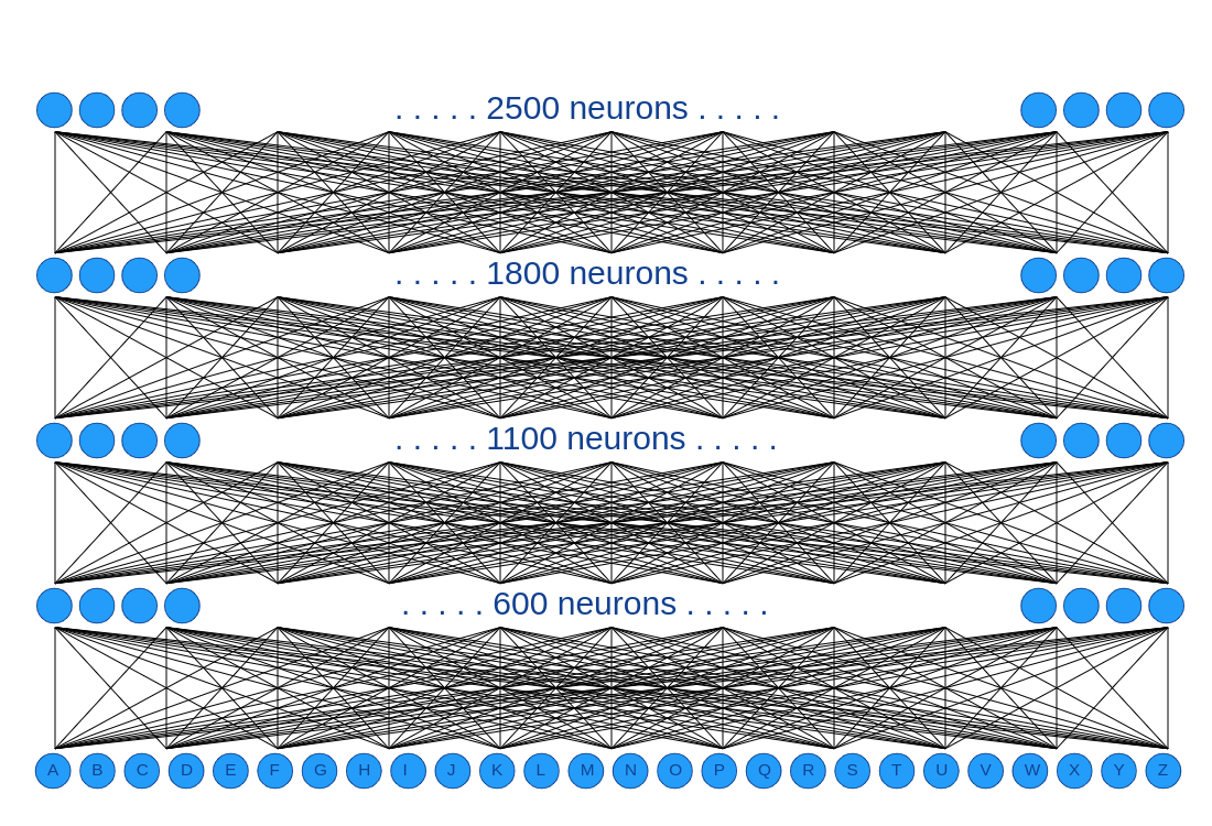
This model takes 2500 neurons as input, so we will now give to it 50x50 images for each character.

It still has 5 layers, and now 26 neurons as output, one by alphabetical character.

We will now use a more consequent data set, we will give 25 images by character:

These images will be converted in one training file, as you’ve already seen before, in order to train the model.

To be more accurate, instead of passing binary data, we will convert the images in normalized vectors. The first step is to get for each pixel the greyscale value (between 0 and 255), and then normalize them to have only values between 0 and 1.

When we have our 26x25 vectors (25 images for each alphabetical character) with the one-hot encoding for each line, our training file is ready.

If now we draw another letter, and automatically do the same operations (vectorization + normalization) before to give it as input of the neural network, it will be able to recognize the letter.

Okay, but how does it really works? A neural network is of course not magical, let’s see how it works behind.

The next part is more theoretical.

Its purpose is to:

Explain how the neural networks really work behind
Introduce you to the common neural network vocabulary and concepts

You can read it quickly and pass directly to the convolutional neural networks (another kind of neural network) if you’re not interested in the mathematical part, but in order to understand the purpose of this other kind of neural network, you’ll need to understand some basics concepts like accuracy, cross entropy loss, or overfitting.

Keras code

You can find the whole sample source code here:

https://github.com/sebferrer/keras-template/tree/main/mlp

How a neural network really works

Degrees of freedom and activation function

When you pass the vector as input of the neural network, a neuron does always the same thing:

It does the weighted sum of all of its inputs,
Adds an additional value (called the “bias”)
Then it passes the value into a mathematical function called an “activation function”

It gives us the following formula for one neuron output: L = activation(X.W + b)

activation(): the activation function
X: the vector of inputs
W: the vector of weights
b: the bias

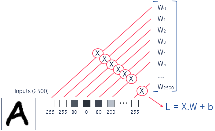
We have then, for each neuron, 2 degrees of freedom:

The bias
The weights of the weighted sum

There can be many functions to use as activation function, but the function must fulfill 2 conditions:

It must not be linear
It must be continuous between 0 and 1

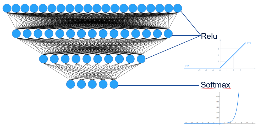
Historically, the activation function has almost always been the sigmoid function, but these last years we recently discovered that the activation of a biological neuron looks more like a relu function than a sigmoid function. After many tests, the researchers in biology discovered that from a certain level, the neurons pass to an activation proportional to the size of the input signals.

That’s why today the relu function is the most used, allowing the model to converge to a more accurate output.

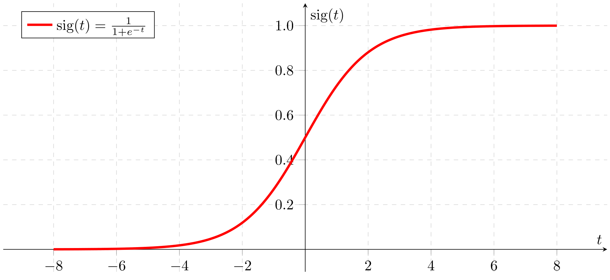
Sigmoid function

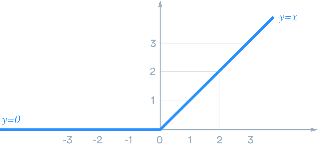
Relu function

That’s what each neuron do, layer after layer.

There’s however an exception for the output layer. We almost always use the softmax function instead of the relu as activation function for the output layer. The softmax is just an exponential function, so after the output neurons has done their weighted sum, they raise the result exponentially, and then we normalize them to have only values between 0 and 1.

This method is used to improve the convergence of the neural network, it widens the gaps between all of the output results. The purpose is to have only values close to 0 (+- 0.1) for every neurons expect for one neuron close to 1 (+- 0.9). We can then interpret it as a probability: the neuron with the output value closest to 1 is the result provided by the neural network.

That’s why it’s called “softmax”, it it highlights the maximum, but without destroying the information. It’s still “soft”.

In our previous example with the characters recognition model, if we have all output neurons with output close to 0 but the second one close to 1, that means that the neural network figured out that the input we passed to it corresponds to the letter “B”.

The first intermediate layer does the weighted sum of the inputs, the layer below does the weighted sum of the previous weighted sums, the outputs of the previous layer, etc…

We can have this result because the neural network was able to converge to the good output, and it was able to do it because the weights and the biases were well chosen.

Okay, but how to chose them? how to direct the weights and the biases in the good direction?

How to direct the degrees of freedom

Accuracy and cross-entropy loss

The entire capacity of a neural network to produce good predictions is based on this.

As we saw earlier, in order to make the neural network able to do a prediction from an input, we need to train it.

The training consists to pass as many inputs as possible in our neural network (like the shapes or the characters in the previous example), and to define an error function, because we already the know the results. Each input is passed with its own one-hot encoded expected input. For each input passed, we set arbitrarily a vector of weights and a bias for each neuron. The result is therefore the output of the last layer with the highest probability. Then we compare this result with the expected result, and we know if the weights and biases were good enough to make the neural network able to do good prediction. That will allow us to establish the error function, and the purpose will to minimize this error function. We call this error function the cross-entropy loss.

This error function is defined by the distance between the output vector (all output neurons values), and the one-hot encoded expected output vector. We could use any distance method, like the Euclidean distance, but the distance that works best today is the cross-entropy distance. That’s why we call our error function the cross-entropy loss.

The cross-entropy consists to multiplying value by value the one-hot encoded expected outputs by the logarithm of the outputs computed by the neural network, and then to do the sum.

Here’s the cross-entropy formula:

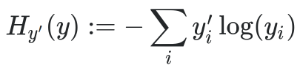
That makes us able to compute the accuracy of the neural network, we call that the evaluation.

The cross-entropy loss decrease and the accuracy increase as the training progresses.

The weights and the biases change in a direction that make the error function decrease.

So now in order to direct the values to the good direction, we need to use an optimizer.

The optimizers

One of the most used is the Gradient Descent Optimizer.

The optimizer will take the error function and compute its partial derivatives in relation to all the weights and the biases of the system.

This involves a huge amount of partial derivative calculation.

Once the calculations are completed, we obtain a vector of partial derivatives.

It’s this vector that we call the gradient.

This gradient points towards the extremum. As we want to minimize cross-entropy, we make it negative, and it then tells us where to direct the values. This then tells us which small delta to add to weights and biases in order to get closer to a value where the error function will be lower.

Finally, when we train a neural network, the whole input dataset won’t be passed only once. It will train again, then again, many times.

We consider that when we train the neural network with the dataset one time, the neural network trained in one epoch. The number of epochs is the number of times you continue to train with the same dataset. So it’s up to us, doing calculations and experiments, to figure out the best number of layers for the neural network, as well as the number of epochs.

These numbers change from a specific need to another.

For a generic use, the number of layers is generally between 3 and 5 for most needs, but some complex neural networks can exceed 80 layers.

For the number of layers as well as the number of epochs, we often find it empirically.

Overfitting

But we have to be very careful when we chose them, it would be a huge mistake to think “more layers and epochs I use, more accurate my model will be. In any case, it can’t make things worse”, because it’s totally wrong. If you use too many layers or if you train your neural network too much (in too many epochs), we will lose the convergence, as well as the accuracy.

This is a common phenomenon, called overfitting.

Vanishing gradient

Now that we have explained what the gradient is, we can understand the problem of the Sigmoid: it has two flat zones on the edges, so having derivatives at these places that tend towards 0. Since the direction we give to weights and biases comes from the gradient, itself composed of partial derivatives, if these derivatives are zero, we no longer have any direction to direct our degrees of freedom.

That’s what we call the vanishing gradient.

This is a phenomenon that occurs when you start stacking layers, which is a problem because stacking layers is part of the machine learning concept.

The Relu function was therefore able to overcome this problem.

But that’s not all there is to say about training yet. Thanks to these methods we were able to make the neural network converge, but we still need to improve the accuracy.

Learning Rate Decay

The first idea to do that is to reduce the step, the delta we use to make the weights and biases progress in the good direction. That will allow the neural network to be more accurate, but this will also make the training slower.

To avoid this inconvenience, we will use the Learning Rate Decay.

This method consists to start very quickly and slow down gradually.

That will allow the deltas to stop varying too much from one direction to another.

Then, we have to take care of the overfitting, and find a way to reduce it.

In order to reduce the overfitting, we will do that we call the regularization, to correct the parts of our calculations that can mislead us.

Regularization and dropout

A very famous regularization method is the dropout, and it’s very simple to understand: we will kill randomly a certain amount of neuron from the neural network (e.g 25%) before to do the training. Then we put all the neurons back in the model, and do the evaluation. We do it again and again, many times. Each time, we restart the operation from the full model.

By killing a neuron, we mean put its value to 0, and slightly raise the other neuron values, to rebalance the average of the vectors.

The reason we’re doing this to regulate the neural network is that a neural network has too much degrees of freedom. Sometimes, some weights and biases can progress in the wrong direction, but if they are significantly outnumbered, the other neurons correct it and keep the convergence. We could say that’s fine while there’s enough neurons to correct, but that also means that we could have a better accuracy. The problem is that we can’t locate the bad neurons and the neurons which correct them.

The dropout method is a simple a very effective method because as at each time we train the neural network there’s a probability for the neurons that corrected the bad neurons to not be there anymore, there’s less chances for the bad neurons to be corrected.

We have now optimized our accuracy and our cross-entropy loss.

For some cases we would have reached the maximum optimization (approximately), but for our example (shapes or characters recognition), we definitely can’t.

Why? Because we did a very brutal operation at the very beginning: we had images/matrix in 2D, and we flatted them. This isn’t really smart, because we lost a huge information: the 2D shape of the matrix.

But we hadn’t the choice, out MLP can take only vectors as input, so what can we do?

The answer is that our type of model is simply not adapted. We need a model that can take a 2D matrix as input.

That’s exactly why the convolutional neural networks were created.

Convolutional Neural Network (CNN)

From 1D to 2D

This time, here’s what our model looks like (still for the characters recognition, 50x50 images):

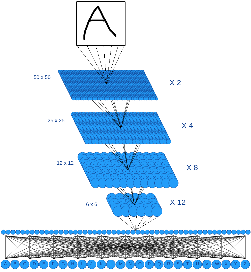
The basis of the principle is the same, but with some differences:

We keep the 2D input information
For a neuron, we don’t do the weighted sum of the entire previous layer anymore
We introduce the concept of channel

Batches and channels

For a MLP, if you remember, each neuron has as input the entire vector of the previous layer outputs, but not this time.

This time, each neuron will have only a patch of the previous layer (4x4 for example) as inputs. We still do the weighted sum of these inputs and we still add a bias, but only with this patch as input.

We continue patch after patch, building another 2D layer of neurons.

Very important: we keep the same weights and the same bias for the all of the patches through the same layer.

With this method, we keep the 2D information, but we don’t have enough degrees of freedom anymore. That’s why we build another layer at the same layer level of this one, but with another weights and bias. It’s like “another version” of this layer.

That’s the concept of channel: the hidden layers won’t be alone anymore, each of them will have a certain amount of another versions of themselves.

Here’s a representation of the inputs for each neurons, patch by patch (here we draw the 2 channels instead of to write “X2”):

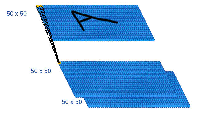
If we zoom a little, that would look like this:

Descriptive Alt Text

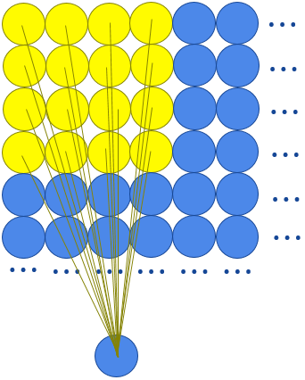
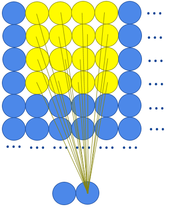
In this example, the same 4x4 weight matrix and the same bias will be used for the whole layer, and the we use another weight matrix and another bias for the second channel.

Using 2D layers and patches allow us to keep every important information, every detail of the shape contained in the image/matrix: pieces of curves, lines, etc…

It’s of course up to us to define the size of the patch (4x4, 5x5, 6x6, …)

If we do this, as we can see above, no matter what number of channel we use, we will generate output layers with the same size as the input layers (it’s logic).

But the purpose of a neural network to converge. To do that, we will simply move the patch not everypixel, but every two pixels (the patch step goes from 1 to 2), we will then obtain output layers twice smaller than the input layer.

We continue to decrease the size of our layers and increase the number of channels, until we’re ready to generate the last hidden layer, a no-convolutional one, fully connected. We are then ready to generate the last output layer whose result will give our prediction. (Cf. our first CNN schema).

The last hidden layer is fully connected, that means that every neuron output of this layer will be the input of every neuron of the output layer, so as a MLP, each neuron has his own weight vector and bias.

If the neural network meets issues to converge (overfitting), that probably means that it doesn’t have enough degrees of freedom. The solution is to use more channels for each layers.

Also, as the MLPs models, adding dropout will help a lot, but only in the fully connected layer. There’s not enough degrees of freedom in the convolutional networks to do that, it would be too risky.

And that’s it! We’re now able to do predictions from 2D inputs with the maximum theoretical accuracy and minimum cross-entropy loss.

Before to finish with the CNNs, it’s good to know that recently we discovered a new method to do a regularization called the batch normalization.

Batch normalization

It consists to divide the whole training dataset in batches, and ensure that the values are in the same scale of values, and that the curves are centered and uncorrelated.

We will be able to compute some statistics for each batch.

For each batch, we will take the output of a neural network layer. For a 100 matrix batch, we sill have 100 output values.

For all of these values, we will compute the average and the standard deviation, and we will modify each layer outputs before to use the activation function.

The modification consists to subtracting the average and to divide by the standard deviation.

For x the initial output computed and x̂ the new output normalized, we can have this formula:

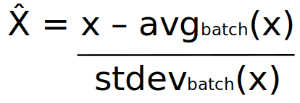
To ensure that we won’t break the outputs that the layer computed, we will add 2 parameters to our new output, so here’s the batch normalization before to use the activation function: BN(x) = αx̂ + β

If the neural networks figures out that it would be a bad idea to transform the output value subtracting the average and dividing by the standard deviation, the parameters α and β will allow us to rewind our calculation. That add 2 degrees of freedom by neuron for our neural network.

As we can cancel each batch normalization, we can ensure that our neural network will be at least as good with the batch normalization as without.

Keras code

The way to build this model with Keras is similar to the MLPs, but this time we take in account the 2D shape of the layers as well as the channels.

Build this model with Keras

 1
 2
 3
 4
 5
 6
 7
 8
 9
10
11
12
13
14
15
16
17
18
19
20
21
22
23
24
25
26


# Image Size
IMG_SIZE = 50
# Number of classes (Number of Persons in Database)
NB_CLASSES = 26

model = Sequential()
model.add(Conv2D(32, kernel_size=(12, 12),activation='linear',padding='same',input_shape=(IMG_SIZE,IMG_SIZE,1)))
model.add(LeakyReLU(alpha=0.1))
model.add(MaxPooling2D((2, 2),padding='same'))
model.add(Dropout(0.25))
model.add(Conv2D(64, (6, 6), activation='linear',padding='same'))
model.add(LeakyReLU(alpha=0.1))
model.add(MaxPooling2D(pool_size=(2, 2),padding='same'))
model.add(Dropout(0.25))
model.add(Conv2D(128, (3, 3), activation='linear',padding='same'))
model.add(LeakyReLU(alpha=0.1)) 
model.add(MaxPooling2D(pool_size=(2, 2),padding='same'))
model.add(Dropout(0.4))
model.add(Flatten())
model.add(Dense(128, activation='linear'))
model.add(LeakyReLU(alpha=0.1)) 
model.add(Dropout(0.3))
model.add(Dense(NB_CLASSES, activation='softmax'))

model.compile(loss=keras.losses.categorical_crossentropy, 
optimizer=keras.optimizers.Adam(),metrics=['accuracy'])

As the CNNs are made to take matrix instead of vectors as input, the inputs are often images.

In order to be able to train and use the neural network with images, here are some functions to convert the images into the matrix we will give to the neural network:

Preparation functions in Python

 1
 2
 3
 4
 5
 6
 7
 8
 9
10
11
12
13
14
15
16
17
18
19
20
21
22
23
24
25
26
27
28
29
30
31
32
33
34
35
36
37


# Set the labels vocabulary for the dictionary. The part before the "_" in the file name will be the label for this image
def label_vocabulary(train_dir):
    labels_dict = {}
    i = 0
    for img in os.listdir(train_dir):
        label = img.split('_')[0]
        if label not in labels_dict:
            labels_dict[label] = i
            i=i+1
    return labels_dict

# Invert keys_values map
def inv_map(map):
    return {v: k for k, v in map.iteritems()}

# Create training data for the images directory
def create_train_data(train_dir):
    X = []
    Y = []
    for img in os.listdir(train_dir):
         word_label = img.split('_')[0]
        label = labels_dict[word_label]
        path = os.path.join(train_dir, img)
        img = cv2.imread(path,cv2.IMREAD_GRAYSCALE)
        img = cv2.resize(img, (IMG_SIZE, IMG_SIZE))
        X.append(np.array(img))
        Y.append(label)
    return X,Y

# Resize the input image and preprocess it
def prepare_image(image, target):
    image = cv2.resize(image, target)
    image = np.array(image).reshape(-1, 50, 50, 1)
    image = image.astype('float32')
    image = image / 255.
    
    return image

Train this model with Keras

 1
 2
 3
 4
 5
 6
 7
 8
 9
10
11
12
13
14
15
16
17
18
19


# Train directory containing the images
train_dir = 'letters'

# Create the dictionary of labels
labels_dict = label_vocabulary(train_dir)

# Create train data
train_X,train_Y = create_train_data(train_dir)
train_X = np.array(train_X).reshape(-1, IMG_SIZE,IMG_SIZE, 1)
train_X = train_X.astype('float32')
train_X = train_X / 255.

# Change the labels from categorical to one-hot encoding
train_Y_one_hot = to_categorical(train_Y)

# Split the training set in validation and training data 
train_X,valid_X,train_label,valid_label = train_test_split(train_X, train_Y_one_hot,  test_size=0.2, random_state=13)

model.fit(train_X, train_label, batch_size=64, epochs=60, verbose=1, validation_data=(valid_X, valid_label))

Test this model with Keras

1
2
3
4
5
6


prediction = {}
prediction['confidence'] = float(max(outputs[0]))
df = pd.DataFrame(data=outputs)
index = df.values[0].tolist().index(prediction['confidence'])
labels_dict_inv = inv_map(labels_dict)
prediction['class'] = labels_dict_inv.get(index)

Output

1

{'confidence': 0.9999970197677612, 'class': '0001'}

So here the class ‘0001’ was recognized, that corresponds to the letter ‘A’

You can find the whole sample source code here:

https://github.com/sebferrer/keras-template/tree/main/cnn

Beyond this blog article

There are many other types of neural network, such as recurrent neural networks (RNN / LSTM) or generative neural networks. Well enough to make this blog post a hundred times longer, but I hope that with this explanation of neural networks via MLPs and CNNs you now have some basics to explore the rest!

All neural network drawings were designed by my own graphic library: BYONND

I also made a neural network studio based on this library: Deep Learning studio

Thanks for reading!